TRANSMISSION OF INTERNATIONAL ENERGY PRICE SHOCKS TO AUSTRALIAN STOCK MARKET AND ITS IMPLICATIONS FOR PORTFOLIO FORMATION

Mohammad Z Hasan¹

¹School of Business, University of Notre Dame Australia, Sydney Campus, Australia

Keywords: Energy price, Stock market, Oil, Volatility transmission, Conditional variance, MGARCH.

JEL Classification:G12, G15, Q4.

Received: 10 November 2016/ Revised: 16 December 2016/ / Accepted: 30 December 2016/ Published: 21 January 2017

Contribution/ Originality:
There is a void in the literature on asymmetric volatility transmissions from the energy market to the stock market. This paper investigates the asymmetric transmission of volatility and shocks in the crude oil, natural gas and coal markets to sectors of the Australian stock market.

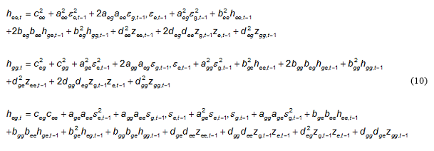
1. INTRODUCTION

The primary objective of this paper is to investigate how volatility has jointly evolved across energy markets and various other asset markets in Australia. We endeavor to estimate the degree to which volatility of one asset market affects the volatility of other asset markets. Specifically, we examine the transmission of international energy price volatility to various GICS sector indices on the Australian stock market. The transmission of volatility from energy markets to the other asset markets is observed via conditional covariance estimated from a bivariate GARCH model. Further, using this conditional variance-covariance matrix, we compute optimal weights and hedge ratios for portfolios consisting two stocks; one from the energy commodity sector and the other from any GICS sector. Studies of energy price shocks and their transmission to other asset markets have critical importance in the construction of investment portfolio. An eminent reason is that the demand for energy is comparatively inelastic¹ . A change in energy price attracts more attention from investors compared with a change in the price of other goods. There is evidence in the literature that major energy price increases in the past have often been followed by severe economic dislocations, suggesting a causal link from higher energy prices to recessions, higher unemployment and possibly inflation (Kilian, 2008). To put it in the context of stock markets, a dramatic shock in the international energy market may spread panic resulting in an outright crash. Therefore, studying the dynamics of international energy prices especially, how they affect stock prices in an individual market is very important for construction and evaluation of portfolios. In particular, this kind of research helps identify which market leads another in price formation. Information (time-varying co-movement of asset returns) obtained from the studies of volatility transmission is used in making optimal portfolio decisions, establishing derivative pricing, and undertaking risk management and hedging. Since energy commodities and GICS indices are potentially attractive investment choices to investors, findings from this type of studies should help investors to work out fund allocation strategies between these classes of asset. Careful investigation of the co-movement of prices of energy and financial assets is equally important for policymakers because understanding how global energy price shocks might be transmitted into the domestic financial system is relevant both to the design and implementation of policies that make contagion less likely.
Although the literature of volatility transmission to stock market is voluminous, a vast majority of these studies consider transmission of oil price shocks to stock markets. In a recent study, Ewing and Malik (2016) examine the volatility spillover between oil prices and US stock market and they observe significant volatility spillover between these two markets. Using BEKK model, Broastock and Filis (2014) document the spillover of oil price shocks to US and Chinese stock markets. For stock markets of emerging economies, Driesprong et al. (2008) observe the spillover effect from the oil price shocks. Literature on volatility transmission from oil market is also extended to sectoral level studies. For example, Duppati and Zhu (2016) study the effect of oil price shocks to sectoral stock returns in Australia, New Zealand, China, Germany and Norway. In another study, Elyasiani et al. (2013) estimate the sensitivity of 10 major US sectors to oil price shocks. It is evident that oil price volatility occupies most of the studies on energy shocks spillover to stock markets. There is a vacuum in the literature relating to volatility transmission from natural gas and coal prices to stocks markets. This study attempts to fill this vacuum. It is important to understand the volatility transmission from coal price to Australian stock market as one-third of the listed companies is related to mining sector and a large number of companies are involved in coal business.  
Studies on volatility transmission to Australian stock market are mainly from volatility of other stock markets. For example, Valadkhani et al. (2008); Brooks and Henry (2000) and McNeils (1993) have found the Australian stock market to covary with the US and UK stock markets. Volatility transmits from the latter into the Australian market. Allowing asymmetric effect and using ARCH class models, Brailsford (1996) finds that volatility innovations in the Australian market influence the conditional volatility of the New Zealand stock market, and vice versa. Using GARCH-M approach, Ratti and Hasan (2013) examine the effect of oil price shocks on volatility in the sectors of Australian stock market and find significant effect for most sectors. In a similar study, Duppati and Zhu (2016) find the exposure of oil price shocks to the sectors in Australian stock market. However, none of these researches considers volatility transmission in these studies. Dean et al. (2010) consider volatility transmission across equity and bond markets in Australia. They conclude that volatility transmits from the bond market into the stock market, but not in the opposite direction. However, these and many other studies address only the linear transmissions of volatility. They do not study the asymmetry of positive and negative shocks. But this study considers asymmetric volatility transmission where conditional co-variances are permitted to react differently to positive and negative innovations of the same size.  We investigate both negative and positive shocks in crude oil, coal, and natural gas returns and study how they transmit to the GICS sector retunes. Thus, we take into account the fact that not only the size of a shock but also the sign of the shock in energy markets is important in determining volatility transmission to stock markets.
Rest of the paper is organized as follows: Section 2 describes the methodology and Section 3 highlights data. Section 4 discusses results while Section 5 concludes the paper. 

2. METHODOLOGY

As mentioned in the previous section, we examine volatility transmission from one asset market to another in terms of conditional (time varying) co-variances obtained via a bivariate GARCH specification. But we begin this section with a brief introduction of univariate GARCH models in order to gain a clear view of the basic idea. GARCH is a popular measure of time-varying volatility because it captures the major characteristics that are commonly seen in the time series of stock returns. For example, volatility has a tendency to converge to a mean rather than diverge to infinity, volatility is high for certain time periods and low for the other periods, and volatility evolves in a continuous manner, that is, volatility jumps are rare –meaning that the volatility is often a stationary process (Tsay, 2010). GARCH volatility captures these characteristics (see (Engle, 1982; Bollerslev, 1986)).
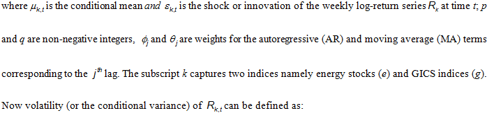
Plainly, GARCH volatility of a demeaned time series is the weighted average of a long-term volatility, known volatility of some past periods and an unknown volatility (shocks or innovations) of some past periods. We said demeaned time series because we are concerned with the volatility of a time series from which the statistically significant trend term or the sample mean is removed, making it a random series. This requires a model for the mean of the time series to be defined before modeling its volatility. We assume that the returns of individual energy stocks and GICS indices are serially correlated and can be defined as a stationary autoregressive moving average (ARMA) process of order (p,q) as specified under:

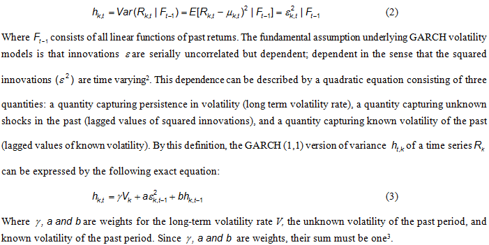
Equation (3) describes GARCH (1,1) variance of a univariate time series. Now we move to see how this equation can be generalized to bivariate cases. We consider bivariate GARCH because we assume that the volatility of a time series is a bivariate process; determined party by its own volatility and partly by that of another variable. For example, we decompose the total volatility of a GICS index into its own volatility and the volatility that spills from an energy stock. The idea of bivariate volatility is analogous to the volatility of a portfolio of two investment choices –in our case one is an energy stock and the other is a GICS index. The unconditional variance (H) of the portfolio is given by (weights are suppressed assuming the variance and covariance are measured in dollars):

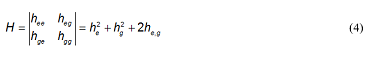
Where the diagonal elements in the metrics are the unconditional variance while the off-diagonals are the unconditional covariance. Recall that, in a univariate case, we model only the conditional variance by equation (3). Whereas, to estimate the conditional volatility of a bivariate time series, we have to specify three equations; one for the variance of the first series (weekly return of energy commodities in our case), one for the variance of the second series (weekly returns of GICS indices) and the third one for the covariance of between the two series.
Application a multivariate GARCH model is a formidable task because of the overload of parameters. Econometricians have proposed several formulations in an endeavor to reduce the number of parametersBollerslev et al. (1988) proposed a formulation where the variables on both the left and right-hand sides are vectors (the upper or lower diagonal part of the variable matrix are stacked in a column). By this formulation, the univariate GARCH (1,1) volatility expressed by equation (3) takes the following form in our bivariate context.

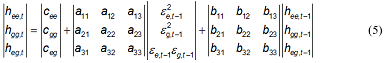
The number of parameters may be reduced by a variation of vech specification known as diagonal vech where the parameter matrices are reduced to diagonal matrices. But restricting the off-diagonal parameters to zero implies that there is no direct volatility spillover from one series to another. Hence, this specification does not fit into our purpose. Furthermore, even though the diagonalization considerably reduces the number of parameters, there is no guarantee that the diagonal vech model will produce a positive variance matrix.        
To guarantee the positive-definite constraint, Engle and Kroner (1995) propose squaring all elements in the conditional variance equation.  This specification is popularly known as BEKK (Baba, Engle, Kraft and Kroner) model. We use this model because it takes into account the dynamic dependence between volatility series –which this study is concerned with.  Many studies have employed BEKK to study spillover of volatility across stock markets. Among the renowned ones are Hamao et al. (1990); Ng (2000); Baele (2005); Mailk and Ewing (2009); Balli et al. (2013).
We consider an asymmetric BEKK GARCH (1,1) model that allows a conditional variance to react differently to negative and positive innovations of the same magnitude. In spirit of Kroner and Ng (1998) we employ the following specification:

3. DATA

We consider three energy commodities and ten GICS indices from the Australian Stock Exchange (ASX). The energy commodities are crude oil natural gas and coal. We take the 1-month future price of West Texas Intermediaries (WTI) as the price of crude oil. While for coal and natural gas prices, we use the 1-month future prices of Henry Hub and ICE Global Newcastle. The GICS indices we consider are energy (XEJ), materials (XMJ), industrials (XNJ), consumer discretionary (XDJ), consumer staples (XSJ), health care (XHJ), financials (XFJ), information technology (XIJ), telecom (XTJ), and utilities (XUJ). The time period we consider is January 2003 to December 2015. Our analysis is based on the time series of the natural logarithm of weekly returns over this period. To obtain these series, we take the natural logarithm of each series of prices and calculate weekly returns as the difference in the logarithm prices over a week. This gives us 679 observations of weekly returns for each commodity and GICS index. The source of all the data is DataStream.

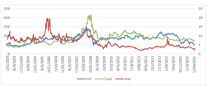
Figure-1. Price of Crude oil, Natural gas, and Coal from Jan 2003 to Dec 2015.

This figure shows energy commodity prices used for the study. Crude oil prices are the 1-month future price of West Texas Intermediaries (WTI), while coal and natural gas prices are the 1-month future prices of Henry Hub and ICE Global Newcastle. All prices are in US dollar. Source of data is DataStream.

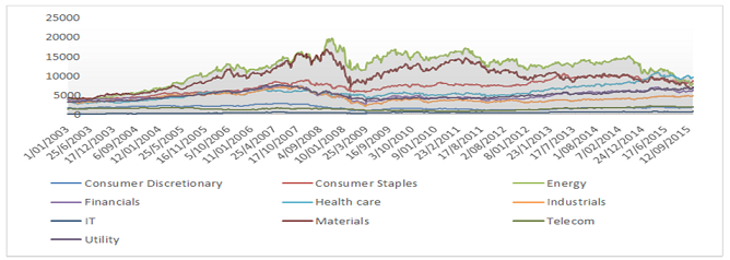
Figure-2.GICS Indices from 2003 to 2015

Source: Datastream

Figure 1 shows the price histories of crude oil, natural gas, and coal during our study period. Crude oil and coal are peaked from 2008 and natural gas prices from 2006. All the prices plummet significantly during the financial recession, showing a significant drop in demand for energy. All energy price returns are significantly volatile during the financial crisis. During 2010, volatility is reduced and there are smoother price movements.

Table-1. The Descriptive Statistics of the Weekly Return of GICS Sectors and Energy Price Returns

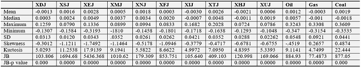
This table reports summary statistics of weekly return of GICS sectors: energy (XEJ), materials (XMJ), industrials (XNJ), consumer discretionary (XDJ), consumer staples (XSJ), health care (XHJ), financials (XFJ), information technology (XIJ), telecom (XTJ), utilities (XUJ), and market (ASX). The sample runs from 2003:03 through 2010:12.

Most GICS sectors have positive weekly mean returns except consumer discretionary, information technology and health. The average returns of GICS sectors are small in comparison to their standard deviation. For energy commodities, gas has negative weekly mean returns during the study period, whereas oil and coal have positive returns. As in the GICS sectors, mean returns of energy prices are smaller than their standard deviation. It is also evident that the mean returns on energy prices are significantly higher than the mean returns of GICS sectors. Among all the energy returns, gas exhibits the highest standard deviation while coal has the lowest deviation. Among the sector returns, the defensive sectors like consumer staples, utilities, and health have lower standard deviations while energy, materials, and financials have relatively higher standard deviations. All GICS sector returns and oil price returns are negatively skewed whereas gas and coal price returns are positively skewed. The skewness of the series implies the data have fat tails. In the case of kurtosis, all the variables show the evidence of leptokurtosis, as the values of kurtosis are greater than three. Hence, none of the return series appears to be normally distributed in terms of skewness and kurtosis. Yet, we check normality using Jarque-Bera (JB) test. The probability values of the JB test indicate that the null hypothesis of is rejected, implying the return series considered in this study are not normally distributed. The following paragraphs present results of more diagnostic tests of the data. Results of these tests speak in favor of the model we choose here. Now we check if a GARCH type model fits our data at all.  A GARCH type model requires the data to have an auto-correlated conditional variance, or the so-called autoregressive conditional heteroscedasticity (ARCH). A quick check for the ARCH effect is to test the squared return series for autocorrelation (see Tsay (2010)). We obtain the autocorrelation coefficients of the squared return series presented in Table 3.

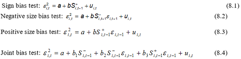
Another common property of volatility is asymmetry in its response to positive and negative shocks. Furthermore, reactions of volatility to big positive shocks and big negative shocks are not the same. To obtain a firsthand idea of these aspects of asymmetry in the volatility, we employ sign and size bias tests proposed (Engle and Ng, 1993).

Table-2. Test of ARCH effect on energy price returns and GICS sector returns

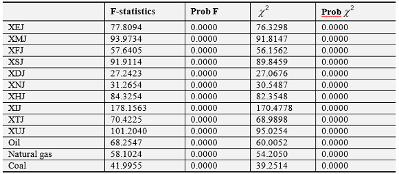
The table reports LM test results to check the presence of ARCH effect in the squared (defined in equation 1) for all return series under consideration. The test considers the null hypothesis that there is no ARCH in the data.

Since we expect positive changes in return of energy to have a larger effect than negative shocks, we use a positive sign bias test. Following Engle and Ng (1993) we run the regressions below:

Individual bias tests are simply the t-tests for the coefficient in the first three regressions. The joint bias test is an F-test of the null hypothesis that all three b parameters in the last regression are jointly zero. Table 3 summarizes the test results. The diagnostic results in the table reveal the presence of asymmetry in the squared residuals of energy returns. In terms of the sign bias test, oil and gas display significant sign bias; this is not evident in coal. In the case of positive and negative size bias tests, the coefficient appears significant at 1% level in the positive size bias tests for oil, coal and gas; and as expected, the coefficient does not appear statistically significant in the negative size bias test. For the oil and gas return series, both sign and size bias tests support the presence of an asymmetric effect, and for the coal return series, the size bias test supports the presence of asymmetry. This justifies our choice of an asymmetric GARCH model.

Table-3. Asymmetric tests of Oil, Coal, and Natural Gas

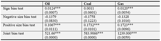
This table reports the estimated coefficients b in equations 8.1 to 8.3. The joint bias test (the forth row) gives the F statistic. Figures in parenthesis are the standard errors. ***, ** and * represent significance at 1%, 5%, and 10% respectively.

Felipe and Diranzo (2005) and Kim and Rogers (1995) suggest checking cross correlations of squared returns before evaluating the volatility transmission between two series. This provides a firsthand idea if there exists any relationship at all between the second moments of two data sets. We estimate the cross-correlations between squared returns of energy and GICS sectors in pairs, considering one energy return and one GICS sector return. The estimated cross-correlations are provided in Table 4. The results reveal that the estimated correlation coefficients of oil with GICS sectors are higher than the correlations of coal and gas with GICS sectors.

Table-4. Correlation between Squared Weekly Energy Returns and Squared GICS Stock Returns

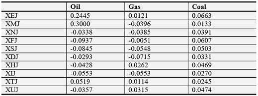
This table reports pairwise correlation between squared returns of the sample over the time period 2003:01 to 2015:12.

4. RESULTS AND INTERPRETATIONS

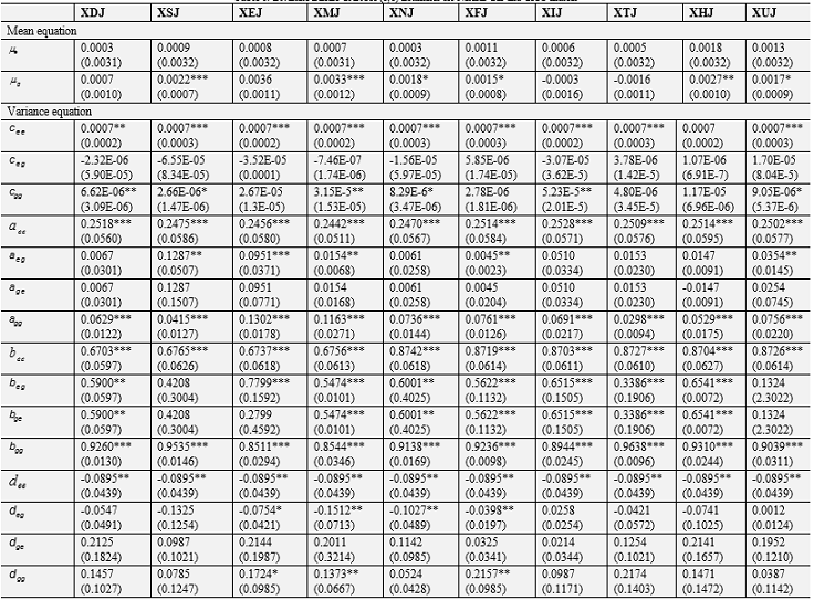
Tables 5, 6, and 7 present results of the study. Each table contains the estimated mean (Equation 1) and the parameters of the variance model (Equation 6) for the bivariate return seriesR_k,t=(R_e,t,R_g,t)  where R_et is the price return of an energy commodity and R_gt  is the return of a GICS index. Recall that we consider three commodities and ten GICS indices. Hence, we obtain thirty equations separated in three tables. For example, Table 5 shows the mean and variance equations for the bivariate return series R_k,t=(R_e,t,R_g,t) where R_e,t is the return of crude oil and R_e,t is the return of the ten selected GICS indices. The first column of the table gives the two means and fifteen parameters of the variance equation for crude oil versus consumer discretionary (XDJ). The second column gives the same for crude oil versus consumer staples (XSJ) and so on. We can read the variance equation for crude oil and consumer discretionary (XDJ) as under where the subscript e stands crude oil and g for consumer discretionary sector, *** and ** are indicators of statistical significance at 1% and 5% respectively and figures in parentheses are the robust standard errors.

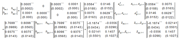
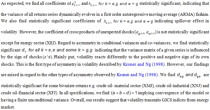
Table-5. Bivariate BEKK GARCH (1,1) Estimates for Crude Oil and GICS Indices

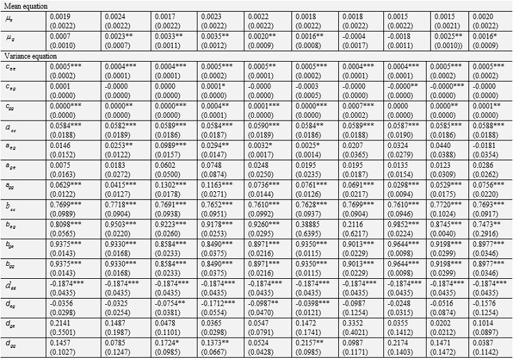
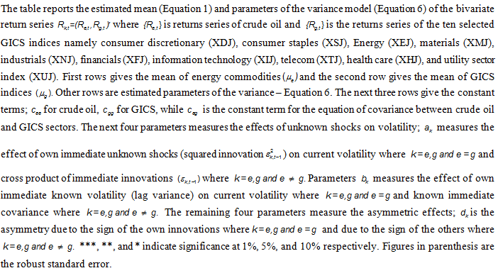
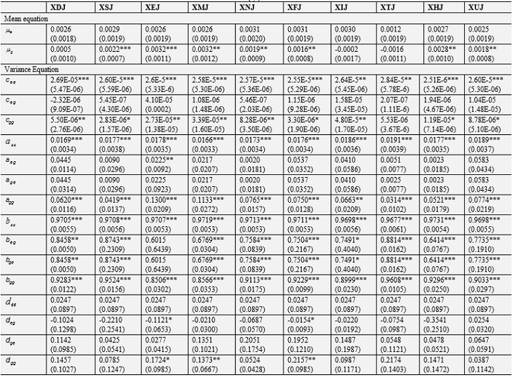
Table-6. Bivariate BEKK GARCH (1,1) Estimates for Natural Gas and GICS Indices

The table reports the estimated mean (Equation 1) and parameters of the variance model (Equation 6) of the bivariate return series Rk,t=(Re,t,Rg,t)   where is returns {Re,t} series of natural gas and {Rg,t} is the returns series of the ten selected GICS indices namely consumer discretionary (XDJ), consumer staples (XSJ), Energy (XEJ), materials (XMJ), industrials (XNJ), financials (XFJ), information technology (XIJ), telecom (XTJ), health care (XHJ), and utility sector index (XUJ). See also the notes under Table 5.

Table-7. Bivariate BEKK GARCH (1,1) Estimates for Coal and GICS Indices

The table reports the estimated mean (Equation 1) and parameters of the variance model (Equation 6) of the bivariate return series Rk,t=(Re,t,Rg,t)' where{Re,t} is returns series of coal and {Rg,t} is the returns series of the ten selected GICS indices namely consumer discretionary (XDJ), consumer staples (XSJ), Energy (XEJ), materials (XMJ), industrials (XNJ), financials (XFJ), information technology (XIJ), telecom (XTJ), health care (XHJ), and utility sector index (XUJ). See also the notes under Table 5.

4.1 Implications of the Study on Portfolio Formation and Hedging

GICS Sector indices and commodities are popular investment choices for investors. Kroner and Ng (1998) mention that the time-varying covariance estimation is crucial for asset pricing, portfolio selection and risk management –the core tasks in finance. Given the estimated time-varying co-variances between energy returns and GICS sectors returns obtained in the previous section, now we calculate optimal portfolio weights for each GICS sector in a portfolio their hedge ratios. We consider a portfolio of two assets comprising (i) any of the three energy commodities namely crude oil, natural gas or coal, and (ii) one of the ten GICS sectors index. The conditional variance of the portfolios is given by Equation (9):

We do not allow short selling, hence, all weights are non-negative and they must sum to one. Weights are calculated using Kroner and Ng (1998) formula as under:

where is the weight for a GICS sector in a portfolio that minimizes variance (risk).

The optimal portfolio weights are given in Table 8. Only the weights of GICS sectors are reported. Here, the investors have a total of $1 invested in one energy commodity and one GICS sector. For example, in the consumer discretionary and crude oil portfolio, the investor should hold 34 cents in consumer discretionary and 66 cents in crude oil for a risk-minimizing portfolio.   
The results reveal that investors have relatively high investments in GICS sectors when one sector is combined with an investment in coal. In the portfolio of coal and one GICS sector, the sector has a weight of 60–70% on average. When the portfolio combines crude oil and a GICS sector, crude oil has the major portion of investment except in the cases of telecom and utilities, where telecom and utilities receive 86% and 60% of the dollar. Again, when the portfolio combines natural gas and one GICS sector, all sectors should have an investment of less than 40%, especially IT and health, which should have 11% and 8% respectively.
Hedging is an important aspect of risk management. In conventional hedging strategy, investors assume constant risks or unconditional covariance between assets. Kroner and Sultan (1993) find this assumption is not realistic, and it is deemed problematic for optimal hedging. They address this problem by using time-varying conditional volatility, and calculate the hedge ratio of two assets as given in the following equation:

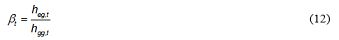
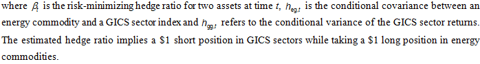
Table-8. Optimal Portfolio Weights and Hedge Ratios

This table reports portfolio weights and hedge ratios based on equations (11) and (12). In a portfolio or hedging, only two assets are considered at once: one from energy and one from the GICS sectors.

Table 8 also presents the hedge ratio for the GICS sector when taking a long position in crude oil, gas or coal. The results reveal that the hedging strategy is expensive, in comparison to the findings of Hammoudeh et al. (2009) and Hassan and Malik (2007). In our case, we need to take a short position of 80 to 90 cents in GICS sectors; Hammoudeh et al. (2009) have a short position of 66 cents on average. Our results imply that hedging is not suitable for taking a short position in GICS sectors in Australia. The hedging strategy becomes effective when the long position is covered by a relatively small position in the short. For example, by following the hedging strategy, one dollar long in crude oil should be shorted by 56 cents in the consumer discretionary sector in the Australian stock market. When taking a long position in oil, financials provides an effective hedge by offering a short position of 55 cents. On the other hand, energy, telecom, and consumer staples are relatively cheap in providing a hedge position, with natural gas in the long position. With coal, all the sectors are deemed to be expensive in hedging, since all GICS sectors need to be shorted at a relatively higher position.

5. CONCLUSION

There is a void in the literature on asymmetric volatility transmissions from the energy market to the stock market. The few studies on volatility transmission from the energy market to the stock market are directed only to crude oil; no study distinguishes between negative and positive shocks in volatility. This reserach investigates the asymmetric transmission of volatility and shocks in the crude oil, natural gas and coal markets to sectors of the Australian stock market. Our analysis uses weekly data from January 2003, to December 2015.
Our results find that volatility transmits from the energy market to the sectors of Australian stock market; however, the converse is not evident. Among the energy commodities, oil, and natural gas are more important than coal for the Australian stock market since a relatively higher number of sectors are affected by volatility transmission from crude oil and natural gas than of coal. Not every sector is affected by shocks in the energy market. The results find that shocks initiated in the energy market transmit mainly to the energy intensive sectors of energy, materials, and consumer staples and financial sectors. The asymmetric response is apparent, suggesting that positive and negative shocks in the energy market are not equally transmitted to the Australian stock market. The results suggest that positive shocks in crude oil and natural gas impact on the material, energy, and financial sectors. Positive and negative shocks in the coal market are not distinctive. In terms of the effect of unexpected news from the oil, gas and coal markets, only the energy and material sectors are responsive to these shocks. The consumer staples sector is only responsive to unexpected news from the natural gas market. The financial and industrial sectors are not responsive to shocks from the energy markets because of the effective risk management strategies taken in these sectors. The volatility of crude oil, natural gas, and coal returns, and of all GICS sector returns, are affected by their own lagged volatility and own unexpected shocks.          
Nowadays, sector index investing is popular, and energy commodities also play an important role in portfolio diversification. Since the covariance between two assets is an important consideration for portfolio construction, research into volatility transmission and conditional covariance between the energy and stock markets provides important insights to investors and market participants. Our results are both useful and timely in providing important information on how specific GICS sectors in Australia behave, and how they interact with the international energy markets. Overall, the findings of this study contribute to building accurate asset pricing models, risk management, hedging and trading policies.

Funding: This study received no specific financial support.

Competing Interests: The author declares that there are no conflicts of interests regarding the publication of this paper.

REFERENCES

Baele, L., 2005. Volatility spillover effects in European equity markets. Journal of Financial and Quantitative Analysis, 40(2): 373-341. View at Google Scholar | View at Publisher

Balli, F., S. Basher and R. Louis, 2013. Sectoral equity returns and portfolio diversification opportunities across the GCC region. Journal of International Financial Markets, Institutions & Money, 25: 33-48. View at Google Scholar | View at Publisher

Bollerslev, T., 1986. Generalized autoregressive conditional heteroscedasticity. Journal of Econometrics, 31(3): 307-327. View at Google Scholar 

Bollerslev, T., R. Engle and J. Woolridge, 1988. A capital asset pricing model with time varying covariances. Journal of Political Economy, 96(1): 116-131. View at Google Scholar | View at Publisher

Brailsford, T., 1996. Volatility spillovers across the Tasman. Australian Journal of Management, 21(1): 13-27. View at Google Scholar | View at Publisher

Broastock, D. and G. Filis, 2014. Oil price shocks and stock market returns: New evidence from the United States and China. Journal of International Financial Markets, Institutions and Money, 33: 417-433. View at Google Scholar | View at Publisher

Brooks, C., 2014. Introductory econometrics for finance. 3rd Edn., UK: Cambridge University Press.

Brooks, C. and O. Henry, 2000. Linear and non-linear transmission of equity return volatility: Evidence from the US, Japan, and Australia. Economic Modelling, 17(4): 497-513. View at Google Scholar | View at Publisher

Dean, W., R. Faff and G. Loudon, 2010. Asymmetry in return and volatility spillover between equity and bond markets in Australia. Pacific-Basin Finance Journal, 18(3): 272-289. View at Google Scholar | View at Publisher

Driesprong, G., B. Jacobsen and B. Maat, 2008. Striking oil: Another puzzle? Journal of Financial Economics, 89(2): 307-327. View at Google Scholar | View at Publisher

Duppati, G. and M. Zhu, 2016. Oil prices changes and volatility in sector stock returns: Evidence from Australia, New Zealand, China, Germany and Norway. Corporate Ownership and Control, 13(2): 351-370. View at Publisher

Elyasiani, E., I. Mansur and B. Odusami, 2013. Sectoral stock return sensitivity to oil price changes: A double-threshold FIGARCH model. Quatitative Finance, 13(4): 593-612. View at Google Scholar | View at Publisher

Engle, R., 1982. Autoregressive conditional heteroscedasticity with estimates of the variance of United Kingdom inflation. Econometrica, 50(4): 987-1002. View at Google Scholar | View at Publisher

Engle, R. and K. Kroner, 1995. Multivariate simultaneous generalized GARCH. Econometric Theory, 11(1): 122-150. View at Google Scholar | View at Publisher

Engle, R. and V. Ng, 1993. Measuring and testing the impact of news on volatility. Journal of Finance, 48(5): 1749-1778. View at Google Scholar | View at Publisher

Ewing, B.T. and F. Malik, 2016. Volatility soillovers between oil prices and the stock market under structural breaks. Global Finance Journal, 29(1): 12-23. View at Google Scholar | View at Publisher

Felipe, P. and F. Diranzo, 2005. Volatility transmission models: A survey. Universitat de València Working Paper. Retrieved from http://www.aefin.es/AEFIN_data/articulos/pdf/A10-2_150613.pdf [Accessed May 22, 2015].

Hamao, Y., R. Masulis and V. Ng, 1990. Correlations in price changes and volatility across international stock markets. Review of Financial Studies, 3(2): 281-307. View at Google Scholar | View at Publisher

Hammoudeh, S., Y. Yuan and M. MacAleer, 2009. Shock and volatility spillovers among equity sectors of the Gulf Arab stock markets. Quarterly Review of Economics and Finance, 49(3): 829-842. View at Google Scholar | View at Publisher

Hassan, S. and F. Malik, 2007. Multivariate GARCH modeling of sector volatility transmission. Quarterly Review of Economics and Finance, 47(3): 470-480. View at Google Scholar | View at Publisher

Kilian, L., 2008. The economic effects of energy price shocks. University of Michigan and CEPR. Retrieved from https://www.aeaweb.org/assa/2009/retrieve.php?pdfid=145 [Accessed May 12, 2015].

Kim, S. and J. Rogers, 1995. International stock and price spillovers and market liberalization: Evidence from Korea, Japan and the United States. Journal of Empirical Finance, 2(2): 117-133. View at Google Scholar | View at Publisher

Kroner, F. and V. Ng, 1998. Modelling asymmetric comovements of asset returns. Review of Financial Studies, 11(4): 817-844. View at Google Scholar | View at Publisher

Kroner, K.F. and J. Sultan, 1993. Time dynamic varying distributions and dynamic hedging with foreign currency futures. Journal of Financial and Quantitative Analysis, 28(4): 535-551. View at Google Scholar | View at Publisher

Mailk, F. and B. Ewing, 2009. Volatility transmission between oil prices and equity sector returns. International Review of Financial Analysis, 18(3): 95-100. View at Google Scholar | View at Publisher

McNeils, P., 1993. The response of Australian stock, foreign exchange and bond markets to foreign asset returns and volatilities. Reserve Bank of Australia Research Discussion Paper No. 9301. Retrieved from http://www.rba.gov.au/publications/rdp/1993/9301.html [Accessed December 12, 2015].

Ng, A., 2000. Volatility spillover effects from Japan and the US to the pacific–Basin. Journal of International Money and Finance, 19(2): 207–233. View at Google Scholar | View at Publisher

Ratti, R. and M. Hasan, 2013. Oil price shocks and volatility in Australian stock retuns. Economic Record, 89(S1): 67-83. View at Google Scholar | View at Publisher

Tsay, R., 2010. Analysis of financial time series. 3rd Edn., New Jersy: John Wiley & Sons.

Valadkhani, A., S. Chancharat and C. Harvie, 2008. A factor analysis of international portfolio diversification. Studies in Economics and Finance, 25(3): 165-174. View at Google Scholar | View at Publisher

---

Footnotes: