


NONLINEAR ANALYSIS OF ECONOMIC GROWTH, PUBLIC DEBT AND POLICY TOOLS

Northeast Normal University (Changchun, China)
ABSTRACT
This paper empirically analyzes the nonlinear relation between real GDP growth per capital and public debt by employing ADL test for threshold cointegration method. Empirical results show that there exists a threshold cointegration relationship between public debt and real GDP growth per capital. In case of the empirical results, cutting public debt could boost economic growth in the long-term. However, the short term variation of public debt makes little impact on real output per capital. Comparatively speaking, human capital and investment rate and trade openness make larger influence on real GDP growth per capital. From the perspective of economic policy, the government should take full advantage of the fiscal policy to cut public debt with the operation space of monetary policy being compressed.
© 2017 AESS Publications. All Rights Reserved.
Keywords:ADL test for threshold cointegration, Economic growth, Public debt, Fiscal policy, Monetary policy, Short-term adjustment.
JEL Classification: H63, E52, E62.
ARTICLE HISTORY: Received:22 August 2016 Revised:26 September 2016Accepted:13 October 2016Published:5 November 2016
Contribution/ Originality:: This study documents the nonlinear relation between economic growth, public debt and policy tools. Based on ADL test for the threshold cointegration method, we find asymmetric adjustments of public debt to economic growth in the short term. Furthermore, fiscal policy could cut public debt more obvious in comparison with monetary policy.
1. INTRODUCTION
In the 1970s, the total amount of public debt of industrialized countries steadily accounted for around 110% of GDP. However in the nearly subsequent 30 years, the private sector and government sector of developed countries continuously issued new public debt which made the growth rate of debt outperform the growth rate of income. Before the outbreak of 2008 financial crisis, the debt/GDP ratio of developed economies had been hiked to 290%. After that, debt/GDP ratio still continues to increase though some developed countries, such as the U.S., employed some economic policies to cut debt of private sector. By the year of 2015, the amount of federal debt reached up to 18.2 trillion dollars, which is the double of that ahead of 2008. The headache problem has troubled not only the U.S. but also the Europe. Before the sovereign debt crisis of Europe in 2011, the public debt of Europe took for about 100% of GDP. While 3 years later, the debt/GDP ratio increased to 120%. The problem of public debt of Japan seems more knotty, whose debt ratio is 260% without considering the amount of private debt. If so, the ratio may reach an astonishing level of 480%.
China is the world’s second largest economy. The variation of debt ratio is also intertwined with the advanced economies. In 2008, the Chinese government implemented the “Save-Plan” which pumped 4 trillion RMB into the market in order to cope with the financial crisis. This action had made the amount of public debt double in just one year. This debt bubble did not attract too much attention by feat of the strong economic growth of China. But in January 2016, the National Bureau of Statistics of China announced the GDP growth rate of 2015 was only 6.9% which had become the lowest point since 25 years. In the context of sluggish economic growth, the problem of public debt of China has emerged.
Economists have long debated the appropriate level of public debt so as to drive the economic growth. Some earlier studies mainly concentrated on the role of debt in developing countries (Smyth and Yu, 1995; Pattillo et al., 2002; Clements et al., 2003) . Some literatures find negative effects of public debt on economic growth. For example, Saint-Paul illustrates the accumulation of public debt would haul the growth rate under the assumption of keeping the capital return constant based on an endogenous growth framework (Saint-Paul, 1992). Besides, some recent papers reveal the threshold effect of public debt to economic growth (Aschauer, 2000; Seo, 2006; Cecchetti et al., 2010; Reinhart and Rogoff, 2010; Cristina. and Rother, 2012) .
When the economy is booming, issuing debt could facilitate investment and consumption and drive economic growth. However when the economy shrinks, excessive borrowing may downgrade the government’s credibility. The constantly default of public debt makes the government have no choice except issuing new debt to counter the previous one. So the public debt ratio expands unceasingly with the cycle repeats.
Unlike previous literatures which employ too much nuisance variables, we make use of ADL test for threshold cointegration method proposed by Li and Lee (2010) to test the long-term cointegration relation between economic growth and public debt at first. Then we investigate the most powerful policy tool to cut debt ratio under the same framework. The two-step method makes us explore the cointegration relation in a more realistic economic environment.
2. DATA SELECTION
Data for the key variables such as real GDP, population, human capital are obtained primarily from the Penn World Table (PWT) version 8.0. Public debt is primarily from the IMF’s Historical Public Debt Database. Investment rate comes from World Bank’s World Development Indicators. Trade, tax, money supply (M2) and government expenditure are collected from CEIC China Economic Database. Annual data are employed in this paper, and the time span is from 1984 to 2011 due to the availability of data.
Table-1. Descriptive Statistics
Maximum |
Maximum |
Average |
Volatility |
ADF Test |
P-Value |
|
Real GDP Growth Per Capita |
11.2022 |
6.2693 |
9.0694 |
1.4855 |
0.6657 |
0.8523 |
Debt Ratio |
33.54 |
0.97 |
12.1486 |
7.9882 |
0.894 |
0.8956 |
Investment Rate |
47.011 |
34.037 |
39.2145 |
3.6627 |
0.9554 |
0.9052 |
Human Capital |
25.7917 |
19.1922 |
22.5048 |
2.1854 |
-0.4619 |
0.5053 |
Trade Openness |
64.769 |
16.6198 |
39.2936 |
13.098 |
0.6395 |
0.8483 |
Interest Rate |
11.34 |
1.98 |
5.4582 |
3.2323 |
-0.8533 |
0.337 |
Inflation Rate |
24.1 |
-1.4 |
5.9893 |
6.5872 |
-1.6137 |
0.0992 |
Tax |
9.1021 |
4.5511 |
6.8475 |
1.2544 |
-0.3931 |
0.897 |
Money Supply |
10.936 |
4.6279 |
8.2913 |
1.7868 |
-2.219 |
0.2356 |
Fiscal Expenditure |
9.2988 |
5.1364 |
7.0003 |
1.2735 |
2.3672 |
0.9999 |
Source:The authors’ estimation.
Additionally, we follow Bekaert to avoid the variable’s endogeneity caused by economic growth’s fluctuations and make use of 5-year average real GDP growth rate as a proxy of economic growth (Bekaert et al., 2000). We take logarithm form of real GDP per capita and then calculate the 5-year average growth rate. This method has been widely accepted. Furthermore, trade openness and investment ratio are calculated by the ratio of trade and investment amount to GDP, respectively. The descriptive statistics are summarized in the Table1.
3. THEORETICAL MODEL OF GDP AND PUBLIC DEBT
In this paper, we follow Checherita-Westphal and Rother (2010) and build a Cobb-Douglas model of economic growth and public debt function which also takes the technical advance into consideration (Checherita-Westphal and Rother, 2010) as follows:
Where, Y, A,L,K and Debt respectively represent the real GDP, technical advance, labor, capital and debt level. What’s more, u is on behalf of the amount which labor contributes to GDP, v represents the public debt in the share of total output.
We can also obtain the following equation:
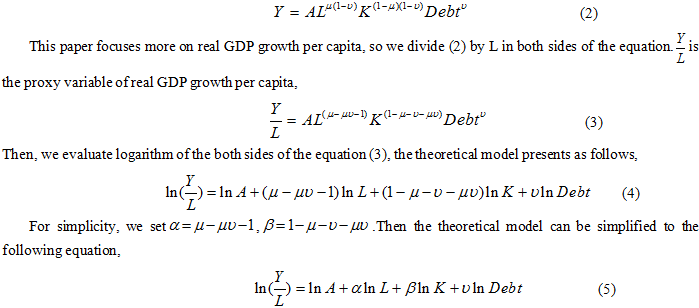
Obviously, there is linear relation between real GDP per capita and public debt. However no official figures of China’s capital amount are available. As an alternative, we choose some other control variables which have close relations to real GDP per capita. So, we can rewrite the equation as,
Whereas, gt and Xt respectively represent the real GDP growth per capita and control variables. A number of literatures have confirmed that high economic growth rate of China has a fixed relation with investment and trade. So we take the two variables into the equation (6). Additionally, some studies reveal that higher human capital could help the country attract more new ideas and facilitate innovation. Thus, we take human capital as the proxy variable of technical advance. In conclusion, the empirical model of real GDP per capita and public debt can be summarized as,
4. ESTABLISHMENT OF EMPIRICAL MODEL
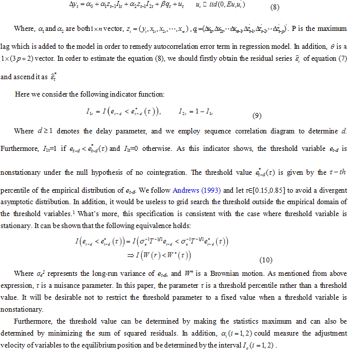
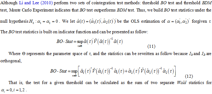
In this section, we follow Li and Lee (2010). The original ADL test for threshold cointegration method can be stated as follow:
5. EMPIRICAL RESULTS
Two parts are involved in this section. Firstly, we need to verify that there indeed exists cointegration relation between real GDP growth per capita and public debt without considering other policy variables. Secondly, we build a policy model which takes public debt and policy proxy variables into account. The aim of the second part is to find the most powerful tool to cut debt.
5.1. The Cointegration Relation between Real Per Capita GDP and Public Debt
At the beginning, the lag order of the model will influence the accuracy of the results. We use the traditional series correlation diagram to decide the optimal lag orders of the model. The figure 1 indicates the optimal lag orders of the series![]() considering the maximum lags of 10. However, we finally let p=1 because of the size of the data.
considering the maximum lags of 10. However, we finally let p=1 because of the size of the data.
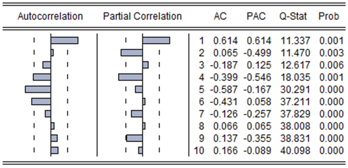
Figure-1. The sequence correlation diagram of ![]()
Source: The authors’ estimation by Eviews 8.0.
Later on, the results of ADL test for cointegration threshold of part 1 are presented as follow:
Table-2.a. BO Test Statistic
1% |
5% |
10% |
|
Critical Value |
44.29 |
38.1 |
35.24 |
BO test statistic |
192.34*** |
Notes: The critical values for BO statistic are tabulated in Table 1 of Li and Lee (2010) paper. ***, ** and
*Significant at the 0.01, 0.05 and 0.1 levels, respectively.
Table-2.b. Cointegration Relation
Variables |
Public debt |
Investment |
Human Capital |
Trade Openness |
Constant |
Value |
-0.1789 |
0.1521 |
0.2138 |
0.0799 |
-3.6838 |
Source: The authors’ estimation.
Table-2.c. Adjustment Coefficient (AC)
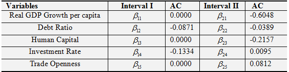
Source: The authors’ estimation.
As Table 2 illustrates, there exits significant cointegration relation among real GDP growth per capita, public debt, investment rate, human capital and trade openness, the cointegration vector is [1,-0.1789, 0.1521, 0.2138, 0.0799 and -3.6838]. However the variation between public debt and real GDP growth per capita is opposite. That’s to say, the accumulation of public debt will reduce real GDP growth per capita. Moreover investment rate, human capital and trade openness would lead to increase of real GDP growth per capita, the coefficients are 0.1521、0.2138 and 0.0799 respectively. Comparatively speaking, trade openness contributes less than the investment rate to the real GDP growth per capita. Whereas human capital may contribute most to real GDP Growth per capita due to the largest coefficient 0.2138.
From the perspective of short-term adjustment coefficient, real GDP growth per capita, human capital and trade openness will not adjust to equilibrium position, characterized by adjusting coefficients are 0 in the interval I. However public debt and investment rate will adjust to equilibrium position, adjustment speed are 0.0871 and 0.1334. In addition, investment rate behave a faster adjustment velocity to equilibrium in comparable with trade openness. However different scenarios occur when the variables are in the interval 2.The variation of investment rate and trade openness will amplify the deviation from equilibrium though with slower rate, merely 0.0095 and 0.0812, respectively. But real GDP growth per capita, public debt and human capital will adjust to equilibrium in the short-term, the speeds are 0.6048、0.0389 and 0.2157. To be noted, the adjustment speed of real per capita GDP is higher than other variables.
5.2. The Cointegration Relation between Public Debt and Policy
As mentioned above, cutting debt ratio can indeed boost economic growth. Given that, we refer to some literatures which are related to cutting public debt by means of economic policy tool. Then, we add the related economic policy variables to ADL test for threshold cointegration model to investigate the most powerful policy tool to cut public debt.
Typically, cutting public debt refers to reduce the ratio of total debt to GDP. There methods could be available to cut the public debt: making the growth rate of public debt smaller than that of economic growth; making the size of the public debt cuts larger than that of economic growth; cutting the total amount of public debt if the economic growth rate keeps steady.
After the World War II, the government of the U.S. cuts as much as 109% of public debt by relying on its strong momentum of economic growth. Without doubt, highly economic growth could be the most helpful tool to cut public debt. However under the background of the excess capacity clearing and structural adjustment in “New Normal”, lower GDP growth rate will definitely occur to China’s economy. Therefore we could only choose the last two methods to achieve the goal. After sorting out relevant literatures, the policy tools can be summarized as follow:
Policy Tool 1: Cutting public debt by employing the fiscal policy
Alesina and Perotti (1996) make use of the data from OECD and illustrate that the adjustment of fiscal structure would be great help to cut public debt. Baldacci and Kumar (2010) note that cutting the government spending and achieving fiscal account surplus could benefit to cutting the public debt.
Policy Tool 2: Cutting public debt by means of inflation
Sargent and Wallace point out that inflation can effectively solve the problem of public debt. Additionally, Aizenman and Marion (2011) note the operability of cutting debt ratio by inflation. They also point out that the government of the U.S. cut 40% of debt ratio benefited from the 10-year long inflation. Some literatures illustrate the reduction of debt ratio could be attributed to inflation, strong economic growth rate and fiscal surplus. However the proportion of inflation is 20%.
Policy Tool 3: Cutting debt ratio by financial repression
Shaw and Mackinnon firstly note the developing countries’ financial repression, which includes the limit of nominal interest rate, high reserve requirements and the cross-border flow of capital (Shaw and Mckinnon, 1976). In addition, lower nominal interest rate could reduce the cost of debt and cut the debt ratio (Reinhart and Sbrancia, 2011).
Given that, we finally choose some policy proxy variables, such as: inflation rate, interest rate, tax revenue, fiscal expenditure and money supply. Then we put those variables and debt ratio into the ADL test for threshold cointegration model and give reasonable policy suggestions. As the method of determining the lag order above, we use the sequence correlation diagram to determine the best lag order of ![]() . As the sequence correlation diagram shows, the best lag order is p=0.
. As the sequence correlation diagram shows, the best lag order is p=0.
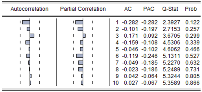
Figure-2. The sequence correlation diagram of ![]()
Source: The authors’ estimation by Eviews 8.0.
After determining the optimal lag order, the results of ADL threshold cointegration show in the table3:
Table-3.a. BO Test Statistic
1% |
5% |
10% |
|
Critical Value |
44.29 |
38.1 |
35.24 |
BO test statistic |
192.26*** |
Notes: The critical values for BO statistic are tabulated in Table 1 of Li and Lee (2010) paper. ***, ** and *Significant at the 0.01, 0.05 and 0.1 levels, respectively.
Table-3.b. Cointegration Relation
Variables |
Inflation Rate |
Interest Rate |
Tax |
Money Supply |
Fiscal Expenditure |
Constant |
Value |
-0.0314 |
-0.1469 |
2.5192 |
-1.5016 |
5.0091 |
-26.726 |
Source: The authors’ estimation.
Table-3.c. Adjustment Coefficient (AC)
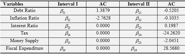
Source: The authors’ estimation.
As table 3 shows, there is significant threshold cointegration relation among debt ratio, inflation rate, interest rate, tax, money supply and fiscal expenditure. The contegration vector is [1,-0.0314,-0.1469,2.5192,-1.5016,5.0091 and -26.7260]. From the perspective of long-term, the increase of inflation rate, interest rate and money supply would be helpful to cut debt ratio, the coefficients are: -0.0314、-0.1469 and -1.5016. The results also prove the results of Aizenman and Marion (2011). However reduction of tax and fiscal expenditure can help cut debt ratio, the coefficient are respectively 2.5192 and 5.0091.
From the perspective of adjustment coefficient, debt ratio will deviate from the balance position in the interval 1. However inflation rate will adjust to balance position, other variables will keep steady in the short-term. Otherwise in the interval 2, debt ratio, inflation rate, tax and money supply would adjust to equilibrium position, adjustment speed are 0.5205、0.1035、24.2620 and 2.0451, respectively. Therefore the adjustment speed to equilibrium of tax is faster than other variables. Whereas variation of interest rate and fiscal expenditure will deviate from the equilibrium, the speed is 0.1987 and 28.5680. Comparatively speaking, the adjustment of fiscal expenditure is more obvious, the coefficient is 28.5680.
6. CONCLUSION
This paper investigates the threshold cointegration relation among economic growth, public debt and public policy based on ADL test. The empirical results show that cutting public debt obviously could benefit to economic growth in the long-term. Additionally, investment ratio and trade openness could also boom economic growth. The results fit the actual performance of China’s economy which heavily depends on investment and trade. Nowadays, another important factor which could be a new path to drive economic growth is human capital which we make it as a proxy variable of technical advance in this paper. The empirical results illustrate the increase of human capital would significantly boom economic growth in comparison with investment and trade. Although investment could also drive economic growth, too large scale of government investment makes investment less efficient. However private sector’s investment is more quality and more innovative, limited funds and less dominance of market make the private sector be edged out of the market. This fact makes the economy have to depend on government investment, and have to face the problems of low yield of the investment and low utilization of factors of production. Most government investment comes from public debt which makes the debt soar along with low investment return. In the context of the vicious cycle, the deep reason is the problem of the mismatch of factors of production among different sectors which results from the unreasonable structure of China’s economy. In order to solve the problem of unreasonable structure, government should refer to supply side. The government should raise the leading role of price in the resources allocation. By the means of accelerating the elimination of the excessive production capacity enterprises and broadening the small enterprises’ financing channels, these methods could make the funds flow to more innovative and higher investment return sectors.
From the perspective of the public debt and economic policy, inflation rate, interest rate and money supply may make negligible impact on cutting public debt. However tax and government expenditure reduction could help to cut public debt with a larger extent. In the long term, cutting government expenditure could make the government free from debt pressure though this action may lead to government expenditure deviate from equilibrium in the short-term. Since November 2014, the inflation rate continued wandering around 2%. The People’s Bank of China (PBoC) announced both reserve requirement ratio reduction and interest rate cut. Furthermore PBoC had also innovated monetary policy tool, such as Standing Lending Facility (SLF), which indicated the policy operation space being compressed. By contrast, the operation space of fiscal policy is still sufficient. The government should promote tax reform, transparency of “The Three Public Consumptions”, normalization of “Anti-corruption” and compression fiscal spending. Despite the use of fiscal policy, especially compressing fiscal spending to cut public debt, could lead to GDP growth deviate from the equilibrium, the cost of this policy is still acceptable.
| Funding: This study received no specific financial support. |
| Competing Interests: The author declares that there are no conflicts of interests regarding the publication of this paper. |
| Contributors/Acknowledgement: I am grateful for the comments and suggestions from anonymous referee and the editor. In addition, I am very grateful to Dr. Shi for his guidance in my graduate phase. I am also very thankful for my parents and Ms. Gao for their meticulous care and attention. |
REFERENCES
Aizenman, J. and N. Marion, 2011. Using inflation to erode the US public debt. Journal of Macroeconomics 33(4): 524-541.
Alesina, A. and R. Perotti, 1996. Fiscal discipline and the budget process. American Economic Review, 86(2): 401-407.
Andrews, D.W.K., 1993. Exactly median-unbiased estimation of first order autoregressive/unit root models. Econometrica, 61(1): 139-165.
Aschauer, D.A., 2000. Do states optimize? Public capital and economic growth. Annals of Regional Science, 34(3): 343-363.
Baldacci, E. and M. Kumar, 2010. Fiscal deficits, public debt, and sovereign bond yields. IMF Working Papers: 1-28. Retrieved from http://ssrn.com/abstract=1669865.
Bekaert, G., C.R. Harvey and G. Bekaert, 2000. Emerging equity markets and economic development. Journal of Development Economics, 66(2): 465-504.
Cecchetti, S.G., M.S. Mohanty and F. Zampolli, 2010. The future of public debt: Prospects and implications. Social Science Electronic Publishing, 68(3): 1–18.
Checherita-Westphal, C.D. and P. Rother, 2010. The impact of high and growing government debt on economic growth: An empirical investigation for the Euro Area. Working Paper No. 56.1237.
Clements, B., R. Bhattacharya and T.Q. Nguyen, 2003. External debt, public investment, and growth in low-income countries. IMF Working Paper: 1-25. Retrieved from http://ssrn.com/abstract=880959.
Cristina., C.-W. and P. Rother, 2012. The impact of high government debt on economic growth and its channels: An empirical investigation for the Euro area. European Economic Review, 56(7): 1392-1405.
Hansen, B., 1997. Approximate asymptotic p-values for structuralchange tests. Journal of Business and Economic Statistics, 15(1): 60-67.
Li, J. and J. Lee, 2010. ADL tests for threshold cointegration. Journal of Time, 31(4): 241-254.
Pattillo, C., H. Poirson and L.A. Ricci, 2002. External debt and growth. IMF Working Paper: 1-49. Retrieved from http://ssrn.com/abstract=879569.
Reinhart, C.M. and K.S. Rogoff, 2010. Errata: Growth in a time of debt. American Economic Review, 100(2): 573-578.
Reinhart, C.M. and M.B. Sbrancia, 2011. The liquidation of government debt. Social Science Electronic Publishing, 68(3): 1–18.
Saint-Paul, G., 1992. Fiscal policy in an endogenous growth model. Quarterly Journal of Economics, 107(4): 1243-1259.
Seo, M., 2006. Bootstrap testing for the null of no cointegration in a threshold vector error correction model. Journal of Econometrics, 134(1): 129-150.
Shaw, E.S. and R.I. Mckinnon, 1976. Money and finance in economic growth and development: Essays in Honor of Edward S. Shaw. New York: M. Dekker.
Smyth, D.J. and H. Yu, 1995. In search of an optimal debt ratio for economic growth. Contemporary Economic Policy, 13(13): 51-59.
Footnote:
1. About the method of grid search, please refer to Hansen (1997).