THE POWER OF A LEADING INDICATOR’S FLUCTUATION TREND FOR FORECASTING TAIWAN'S REAL ESTATE BUSINESS CYCLE: AN APPLICATION OF A HIDDEN MARKOV MODEL

Yun-Ling Wu¹ --- Cheng-Huang Tung² --- Chun-Chang Lee^3†

¹Lecturer, Department of Real Estate Management, National Pingtung University, Taiwan , ²Associate Professor, Department of Computer Science and Information Engineering National Pingtung University, Taiwan , ³Professor, Department of Real Estate Management, National Pingtung University, Taiwan

Keywords: Real estate cycle, Real estate cycle leading indicator, Asymmetry, Duration, Hidden Markov model, Taiwan real estate research center.

Received: 19 July 2016/ Revised: 21 September 2016/ Accepted: 19 October 2016/ Published: 5 November 2016

Contribution/ Originality

This paper uses the HMM to capture the optimal path of state transition to observe the trends of fluctuations of out-of-sample data. The results confirm that trends of the real estate business cycle fluctuations are asymmetric and that the average duration of recession periods is longer than that of expansion periods.

1. INTRODUCTION

The long-term trends of the business cycle in the real estate market and how to predict fluctuations in that business cycle are subjects of great topical concern in macroeconomic analysis and decision making. Tvede et al. (2008) found that, according to a conservative estimate, construction activities account for 10% of global GDP, of which one fifth comes from stable market fluctuations in the public sector and the rest results from significant periodic business cycle fluctuations. In other words, when activity in the real estate market decreases by 33%, there will be a 3% decrease in GDP, with that decrease not including the wealth spillover effects caused by the plunge in real estate prices. In addition, market observations over the past several decades and even century suggest that there are repeated business cycle fluctuations in the real estate markets around the world and that real estate market fluctuations often lead to considerable fluctuations in raw material prices. Hence, monitoring the trend of real estate market cycle fluctuations is an important activity in the field of macroeconomic research.

Previous studies on business cycles can be categorized in two ways. First, in previous studies aimed at analyzing the real estate business cycle and its causes, researchers have applied proxy variables such as vacancy rates (Grenadier, 1995; Gordon et al., 1996) and real estate rental growth rates (Mueller, 1999) in their analyses. Second, the relationship between residential housing market price and quantity (Edelstein and Tsang, 2007) imbalances in real estate market supply and demand (Roulac, 1996) investment expectations (Huang, 2013) and the mortgage loan supply and asset price relationship (Arsenault et al., 2013) have been used to describe the causes of and changes to the real estate business cycle. However, those studies only describe the business cycle fluctuations or causes of fluctuations without comprehensively explaining the implications of the real estate business cycle. Moreover, some studies have discussed the real estate business cycle and macroeconomic relationships, or the mutual influences of relevant industries (Pritchett, 1984; Clayton, 1996; Goetzmann and Wachter, 2000; Kan et al., 2004; Leung, 2007; Huang, 2013). However, research on the composite indicators of the real estate business cycle is still relatively rare.

In order to directly quantify real estate business cycle fluctuations, recent studies have adopted the composite real estate index. Krystalogianni et al. (2004) used the leading composite index to predict the features and performance of the British commercial real estate cycle. Lee et al. (2009) applied the real estate leading composite index and Markov-switching model to explore the change in the real estate business cycle turning points. They found that the performance of the leading composite index for identifying real estate business cycle turning points is good. Although state transitions were excessively frequent and there were some disparities in terms of the durations of business recession and expansion periods, the model fitness performance and application were both found to be good. It was concluded that the composite index is superior to the single series for understanding business cycle fluctuations.

Many recent studies on macroeconomic cycles or real estate business cycles have focused on the observation of business turning points (Scott and Judge, 2000; Baum, 2001; Barras, 2005) and business duration periods. For the measurement model, the Markov switching model proposed by Hamilton (1989) has been the most widely applied, having been applied in various studies such as those of Hamilton (1989); Pelagatti (2001); Krolzig (1997) and Cruz (2005). The main advantage of the Markov-switching model is that it can capture the random changes of the business state over time through a group of unobserved state factors in the model setting mechanism. Moreover, the model can slightly modify the model pattern with different data patterns, such as the Markov model of intercept changing with state (Hamilton and Susmel, 1994) the Markov model of variance changing with state (Cai, 1994; Hamilton and Susmel, 1994; Gray, 1996) or a variety MSVAR (Markov-switching vector auto-regression models) (Krolzig, 1997). Hence, the application and analysis process of the model is more flexible and practical. The Markov-switching model is mainly dominated by a group of unobservable states and the random transition jumping mechanisms between those states. The state setting is the unobservable variable and is able to describe the features of the state random change. However, in the preset viewpoint, if the state is set as unobservable, it is not consistent with the observable data. As such, during the analysis process, it may be able to capture the state of random change but not able to observe state features, thereby losing a more accurate estimation of state path switching probability. As a result, it may lead to estimation error in estimating the trend of business cycle fluctuations.

The state random switching theory of the Markov-switching model in the framework of probability theory, namely the hidden Markov model (HMM), can be regarded as a double-embedded stochastic process (Huang et al., 2001). A complete HMM consists of two random processes: one layer is the hidden unobserved state switching series corresponding to a pure first-order Markov process, while the other layer is the observable random series in the hidden state. In the Markov - switching model, although random state switching series cannot be observed, through the observable series of state, a hidden Markov model can predict the originally unobservable state switching series probability. As the hidden state series is transformed into the observable state feature series, this model is known as the HMM.

The HMM was first applied in the late 1970s for the identification of sound signal fluctuations (Baum and Petrie, 1966) and is now widely used in engineering, genetics and other fields, such as communications audio classification and speech recognition, with considerable research achievements. According to Hassan and Nath (2005) the HMM model has the following advantages: (1) a strong statistical basis; (2) the ability to handle new information robustly; (3) the capacity to calculate and forecast similarity modes more efficiently. In recent years, the HMM model has been applied in economic, financial, and management fields, including economics in general (Leng and Wang, 2014) and the study of financial series fluctuations more specifically (Gregoir and Lenglart, 2000; Hassan and Nath, 2005; Korolkiewicz and Elliott, 2008; Oguz and Gurgen, 2008; Liu, 2010; Roamn et al., 2010; Zhu and Cheng, 2013). In the management field, it has been used to study customer relations management (Bouchaffra and Tan, 2004; Shen and Zhao, 2006; Netzer et al., 2008; Sepideh and Aaghaie, 2011) and online purchasing behaviors (Wu et al., 2005).

By following the current literature on the forecasting of real estate business cycle fluctuations and measurement models, based on the developed Markov-switching model, this study uses the real estate business cycle leading indicator composite index (footnotes 1) released by the Taiwan Real Estate Research Center to establish a discrete hidden Markov-switching model (discrete HMM; HMM with discrete output observations), in order to capture unobservable state implications. It is expected that the model will be able to predict the trends and changes in the real estate business cycle, as well as detect business turning points and state duration periods.

The remainder of this paper is organized as follows. Section 2 introduces the HMM theory and model parameter estimation; Section 3 explains the data description and analysis, as well as the features extracted from the economic cycle leading indicators series to comply with HMM model setting principles and ideas; Section 4 discusses the empirical results analysis; Section 5 offers conclusions.

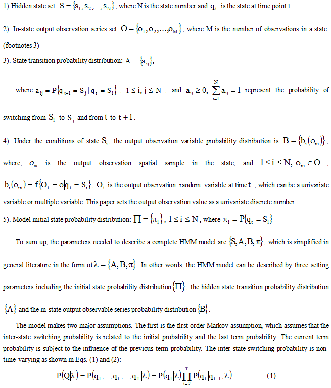
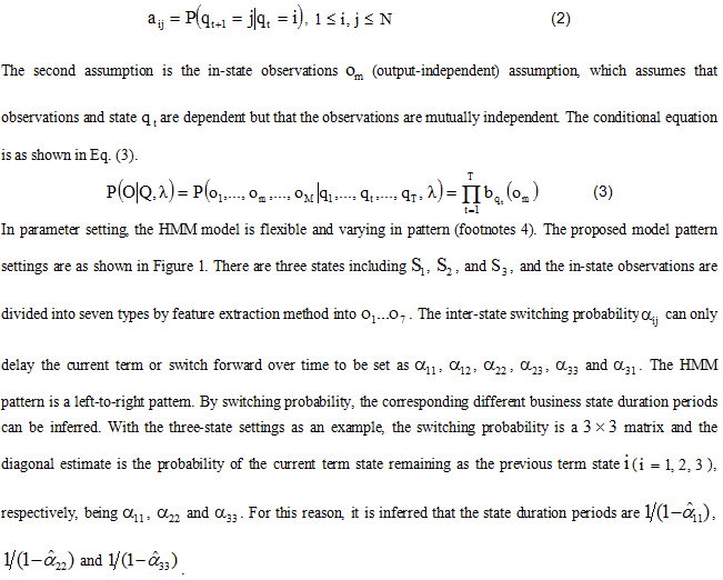
2. HIDDEN MARKOV MODEL AND MODEL PARAMETER ESTIMATION

In previous studies, economists have developed a series of non-linear econometric models by describing the changing process of linear model parameters. The state transition model (regime switching model) can process multiple jumping processes of the parameters (footnotes 2). In order to observe the real estate business cycle leading indicator’s trend characteristics and the predictability of series fluctuations, this paper uses a non-linear HMM model as the measurement research tool. The model and parameter estimation results are as explained in the sections that follow.

2.1. HMM

In terms of the overall parameters and random concepts, the HMM can be divided into two parts. The first part can be described as a Markov chain to generate hidden state random series; the second part of the random process is described by the distribution of the observation variable probability in the state. The basic elements are as shown below (Huang et al., 2001; Koskinen and Öller, 2004):

The left-to-right pattern is a type of generalized HMM pattern. The generalized HMM model pattern means that the inter-state switching probability can switch randomly without limitation. The main difference between the left-to-right pattern and the generalized pattern is that the inter-state switching probability can delay the current term or switch forward only (i.e., it cannot switch backward). The concept of such a setting mainly comes from the notion of moving forward in time and the idea that the state switching path will naturally jump forward. As shown in the above HMM model, the observation output sample space and probability distribution in hidden space may have different setting patterns according to the literature. This paper emphasizes the capability of the HMM model to capture the inter-state switching. Hence, it is set as a univariate discrete observation data pattern.

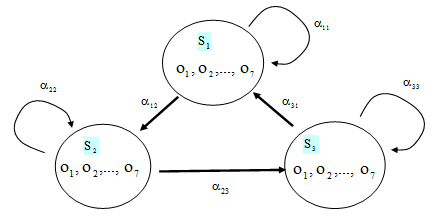
Figure-1. The HMM model pattern proposed in this study

Source: Compiled by this study.

2.2. HMM Model Parameter Estimation Method

There are three basic problems to solve by using the HMM model to obtain the optimal parameters, namely, model training, hidden state optimal path estimation, and the computation of the maximum likelihood estimate (Baum and Petrie, 1966). The estimation method is briefly described as follows:

1). Computation of maximum likelihood estimate

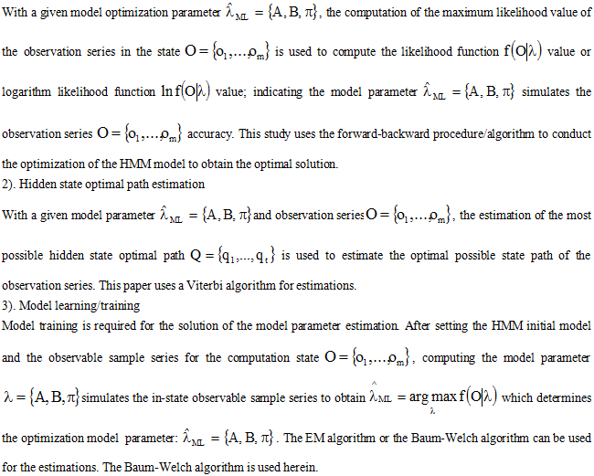
In the evaluation of the model predictability, this paper uses expected loss function principles of turning point error (TPE) and mean squared error (MSE) to evaluate the forecasting errors between the actual observation values of the leading indicator and the estimated predicted values by using the HMM model to illustrate the performance of applying the HMM model in predicting the trends of the real estate business cycle leading indicator fluctuations. The two inspections can simply and directly compute the expected loss or expected cost error between the predicted values and the actual values.

3. DATA SOURCE AND ANALYSIS

The data used in this study were sourced from the real estate business cycle leading indicator composite index values from 1971 Q1 to 2009 Q4 released by the Taiwan Real Estate Research Center, a period including 156 samples of seasonal data. The Center releases data regarding the trends of the real estate business cycle via quarterly reports and elaborates on the compilation of economic cycle leading indicator series in the appendices of those quarterly reports. As the series data contained in the economic cycle leading indicators have different characteristics, after the verification of the quarterly and trend statistics method, all the contained series have been de-trend adjusted, while some data are seasonally adjusted by X12 software. The construction stock price index representing investments, the construction loan credit balance change representing production, and the CPI representing transactions have been adjusted according to the trend. In addition, the GDP and monetary supply values in the investment dimension have also been revised according to the de-trend adjustment and seasonal adjustment.

According to the previous literature, when analyzing a relevant time series by using an empirical model, the data should consist of a stationary series (footnotes 5) for parameter estimation and statistical inference. This paper conducts the ADF (augmented Dickey-Fuller test) unit root test of economic cycle leading indicators in advance to determine whether the series data are stationary. On the assumption of null hypothesis with a unit root, the ADF test confirms that the real estate business cycle leading indicator has a unit root, suggesting that series data are non-stationary. After the first differentiation of the data, this study conducts the ADF unit root, finding that the economic cycle leading indicator series at the 1% significance level rejects the null hypothesis after the first differentiation. In other words, after the first differentiation, the economic cycle leading indicator series is stationary. Therefore, this study adopts the first differentiation series of leading indicator for analysis.

Regarding the setting of the HMM model, the number of states should be set in the beginning. According to the purpose and pre-concept, the number of states can be increased or decreased independently. Most of the previous studies on the overall business cycle or real estate business cycles have described business cycle fluctuations in terms of two states (Lee et al., 2009). Some research has used three states. For example, Cruz (2005) pointed out that the expansion and shrinkage stages of the three-state business cycle model described in previous studies was relatively similar to the turning points released by the NBER (National Bureau of Economic Research). The proposed model sets three business states, namely, market recession, market of no significant change, and market expansion. The setting of two states may result in excessive range to capture the feature information in the HMM model. In the estimation of the state switching probability, inter-state switching will be too slow to lead to an excessively lengthy duration period for each state. As a result, it is difficult for the HMM model to capture in-state features.

Second, with regard to the observable information value of each in-state type and the corresponding univariate business leading composite index, the univariate variable is set as discrete. This study uses the feature extraction method to process by dividing the information of the economic cycle leading indicators series by change into {significant increase, general increase, modest increase, small change, modest decrease, general decrease, significant decrease) output signals. Therefore, from 1971 Q2 to 2009 Q4, the leading indicators’ discrete observable data were extracted. This paper applies the feature extraction method in a manner similar to the concept of compiling business countermeasure signals (footnotes 6) to categorize series into a number of features by change. In addition to the emphasis on the application of the HMM model in the forecasting of the trends of business cycle fluctuations, it is expected to highlight the market state fluctuations’ degree and data switching features including business data expansion, recession, and others. Huang et al. (2001) extracted Dow Jones industrial average index features to represent the bull market, bear market, and fluctuations market of no change. Unlike the five types of business monitoring indicators, that study extracted seven types of trend signals of features fluctuations, expecting to further categorize the fluctuation degree of the leading indicator to observe more characteristics of the trends of the business cycle fluctuations. As mentioned above, Huang et al. (2001) argued that the continuous data contain a considerable degree of information despite the feature extraction of discrete data. However, if they are further divided into nine types or more, the value of each change is too small and the distinguishing of features will be too insignificant. As a result, it may result in excessively frequent jumping of state switching path probability. Therefore, this paper sets seven types of features.

To measure the forecasting capabilities of the HMM model against the trends of fluctuations, this paper divides the business leading composite index series (1971 Q2~2009 Q4) into two groups. One group consists of the in-sample (1971 Q2~2008 Q4) samples; this group, with a total number of 152 samples, is used as the training data for parameter estimation. Another group is the out-of-sample (2009 Q1~2009 Q4) observation data for 4-step-ahead forecasting. In addition, by using the rolling window sampling method (footnotes 7), with 4 seasons as a unit time length, the sample data are sorted out by time. The one-term lag data start with 1971 Q2 and develop at the interval of one season to 2008 Q4 to result in a total of 148 pattern training samples. The rolling window for the preprocessing of the observation samples can increase the number of samples to improve the accuracy of the parameter estimation. Meanwhile, it is expected to simulate the similar fluctuation path pattern series by using the in-sample samples as the four-term pattern samples in the forecasting of out-of-sample 4-step-ahead forecasts to improve forecasting accuracy.

4. ANALYSIS OF EMPIRICAL RESULTS

This section contains two parts. The first part is the description and analysis of the HMM model estimation and 4-step-ahead forecasts. The second part further elaborates on the forecasting capability of the application of the model in the trends of the economic cycle leading indicators out-of-sample fluctuations.

4.1. Analysis of HMM Model Estimation Results

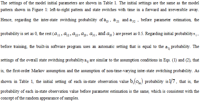
The settings of the model initial parameters are shown in Table 1. The initial settings are the same as the model pattern shown in Figure 1: left-to-right pattern and state switches with time in a forward and irreversible away.

For model training and program computation, this paper uses the built-in HMM program of MATLAB 7.0 software to obtain the parameter optimal solutions by iteration computation of the logarithm maximum likelihood value. Figure 2 illustrates the iteration time’s curve of the logarithm maximum likelihood during the optimal parameter estimation process. When the tolerance rate is 0.000001, the model parameter estimation converges when the iteration times are 432 during the model parameter estimation, and the logarithm maximum likelihood values are -1048.6.

Table-1. Initial parameter settings of the model before training ()

Parameter	Initial setting (before training)
			State 1		State 2					State 3
			0.5		0.5					0
	State 1		0.5		0.5					0
	State 2		0		0.5					0.5
	State 3		0.5		0					0.5
			Significant increase	General increase			Modest increase	Small change			Modest decrease	General decrease	Significant decrease
	State 1		0.14286	0.14286			0.14286	0.14286			0.14286	0.14286	0.14286
	State 2		0.14286	0.14286			0.14286	0.14286			0.14286	0.14286	0.14286
	State 3		0.14286	0.14286			0.14286	0.14286			0.14286	0.14286	0.14286

Source: Compiled by this study.

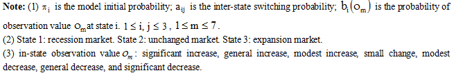
Figure-2. The iteration times curve of the logarithm maximum likelihood of the discrete HMM model

Source: Compiled by this study.

The average duration period of business in the state of recession (state 1) is 5.23 seasons, the average duration period of business in the state of market of no change (state 2) is 1.69 seasons, and the average duration period of business in the expansion state (state 3) is very short. From the perspective of state 1 and state 2 switching probability, the state is continuous, which confirms the characteristic of Taiwan’s real estate market business state being difficult to change and supports the viewpoint of continuous business state. The state 3 (expansion market state) probability estimation suggests that it is difficult to remain in the same state. This paper infers that the setting of the HMM model shifts from left to right. As a result, the probability shifts from state 3 to state 1. In addition, the leading indicator trends in Figure 3 suggest that the trends in the expansion stage are steep and that the downward fluctuation sections are frequent. Hence, the trend deepness in the expansion state is relatively less steep as compared with the deepness in the state recession period. Therefore, it is relatively easier to shift to the recession period. The probability value of state 3 suggests that it is unlikely to remain in state 3. The estimation verifies that the period of business recession is longer than the expansion period.

The above estimation results of the business average duration period suggest that the real estate business cycle’s recession and expansion periods are asymmetric (footnotes 9). In this respect, the findings of this study are consistent with most of the available empirical results for the overall business cycle or the real estate business cycle, indicating that expansion periods and recession periods have asymmetric trends. The real business cycle model is considered to be subject to the influence of the same random variables in business expansion period and recession period states, and thus they have the same degree of fluctuations and the same dynamic characteristics. However, Figure 3 suggests that the trend of increasing real estate business cycle leading indicator data during the period from 1971 to 2009 is steeper and shorter in duration. On the contrary, the trends of the decreases in most indicators are less steep and last longer. The long-term trends of time series data are consistent with the empirical results.

According to the estimation results, when the market is in the recession state, the total probability of observations of decreases in leading indicators (i.e., modest decreases, general decreases, and significant decreases) is 0.2065. When the market is in a state of no significant change, the probability of the trend change observation (small change) is close to 50%, and up to 0.4136. When the market is in a state of expansion, the feature value of the in-state observation value general increase is 0.5213. Roughly speaking, the in-state feature value probability distribution meets our expectations, as the features in the expanding market state (state 3) (significant increase, general increase and modest increase) may concentrate on the observation feature of the modest increase. The probability of the occurrence of the two observation features is almost 0. This may be caused by the steep trends of the real estate business cycle leading indicator in the expansion period, and the in-state feature closer to the boundaries of other states can be more easily captured by the small change features of state 2 in probability. As a result, it is difficult for the model to capture in the expanding market state the probability of two features including significant increase and general increase but concentrate on the boundary section of state 2 features. Another possible reason is that the samples are not categorized by smaller features and thus the abnormalities of each in-state feature can easily affect the bias of the probability estimation.

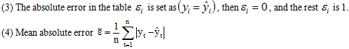
In 4-step out-of-sample forecasting, through the known in-sample observation data, the discrete HMM model is established to allow the known out-of-sample forecasting observations and known in-sample observation data to have a similar pattern and similar statistical characteristics. The forecasting results error rate is as shown in Table 3. According to the absolute error and mean absolute error ratio of the simple state estimates, the forecasting accuracy of the out-of-sample data is not satisfactory, which is as expected. According to real estate business cycle leading indicator trends as shown in Figure 3, the indicator has been considerably decreasing since 2008. There is a possibility of series structural change.

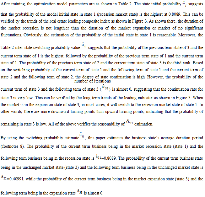
Table-2. After HMM training, model () parameter

Parameter	Optimal parameter (after training)
			State 1				State 2			State 3
			0.8089				0.1911			0
	State 1		0.8089				0.1911			0
	State 2		0				0.40991			0.59009
	State 3		1				0			5.9788e-057
			Significant increase	General increase	Modest increase			Small change	Modest decrease		General decrease	Significant decrease
	State 1		0.1371	0.1176	0.1252			0.4136	0.1283		0.0782	0.0000
	State 2		0.0000	0.0000	0.2588			0.0000	0.0478		0.3628	0.3307
	State 3		0.0000	0.0000	0.0000			0.4787	0.5213		0.0000	0.0000 parameter

 

Source: Compiled by this study.

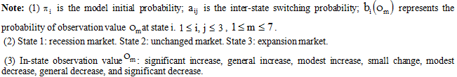
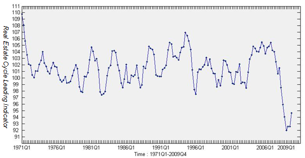
Figure-3. Trends of the real estate business cycle leading indicator (1971Q1~2009Q4)

Source: Compiled by this study.

Table-3. HMM model 4-step out-of-sample forecasting results - mean absolute error rate

Forecasting period	Actual state value	Predicted state value	Absolute error	Mean absolute error(%)
2009 Q1	1	2	1	100 %
2009 Q2	3	2	1
2009 Q3	2	3	1
2009 Q4	3	1	1

Source: Compiled by this study.

Note: (1) In this study, the business state is divided into three types: state 1: recession market. State 2: unchanged market. State 3: expansion market.

(2) Forecasting period: 4-step-ahead forecasts.

This paper further examines the model-estimated data of each year, and deletes the samples of 2008-2029 suspected of structural changes. The total sample HMM model is then applied in the estimation of parameters, and the means absolute error rate is applied in the detection of total sample of each year in four-step forecasting as shown in Table 4. The results are consistent with those of Wu (2009). The mean estimation error rate of the total sample is 44.90%; the accuracy of forecasting samples out of the four-step forecasting (2007Q1-2007Q4) is up to 75%. It is concluded that the HMM model has good accuracy in forecasting fluctuations of the business cycle leading indicator. The results validate the inference of this study. In the period of 2009 Q1 to Q4, there are structural changes in Taiwan’s real estate business cycle leading indicator. Previous literature (Rau et al., 2001; Chen, 2006) on the overall business cycle of Taiwan indicates that structural change occurred during the 1990s. In the field of real estate business cycle research, many articles on the measurement of the real estate business cycle by housing price, such as those by Chen (2003) and by Peng et al. (2004) argue that housing prices did undergo structural changes. However, to avoid divergence of research topics and to simplify the model to highlight the characteristics of the HMM model for capturing the jumping state, the topics of structural change are not considered and explored in this study.

Table-4. HMM model forecasting results of total sample in each year-mean absolute error rate detection table

Period of sample forecasting	Mean absolute error rate (%)	Period of sample forecasting	Mean absolute error rate (%)	Period of sample forecasting	Mean absolute error rate(%)
60Q2-Q4	0	73Q1-Q4	75	86Q1-Q4	0
61Q1-Q4	25	74Q1-Q4	25	87Q1-Q4	75
62Q1-Q4	75	75Q1-Q4	25	88Q1-Q4	75
63Q1-Q4	25	76Q1-Q4	0	89Q1-Q4	50
64Q1-Q4	100	77Q1-Q4	25	90Q1-Q4	25
65Q1-Q4	50	78Q1-Q4	50	91Q1-Q4	25
66Q1-Q4	75	79Q1-Q4	50	92Q1-Q4	75
67Q1-Q4	75	80Q1-Q4	25	93Q1-Q4	50
68Q1-Q4	50	81Q1-Q4	50	94Q1-Q4	75
69Q1-Q4	75	82Q1-Q4	0	95Q1-Q4	50
70Q1-Q4	75	83Q1-Q4	25	96Q1-Q4	25
71Q1-Q4	25	84Q1-Q4	0
72Q1-Q4	50	85Q1-Q4	25

Source: Compiled by this study

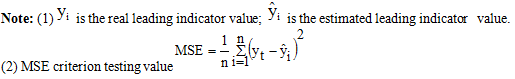
This paper further uses the MSE criterion to estimate the accuracy of estimation by determining the degree of error as indicated by the difference between the actual value and the forecast value of the business indicator. The total MSE result is 1.0148, as shown in Table 5, where is the leading indicator value deduced from the optimal path by the estimation of the HMM model. Before the application of the HMM model, this study has extracted the features of the economic cycle leading indicators for intermittent classification. In the process, to extract features, the category average number is estimated. Hence, is the average feature category deduced from the optimal path of forecasting.

Table-5. HMM model 4-step-ahead forecasts-MSE criterion test

Forecasting period	Actual leading indicator value ()	Estimated leading indicator value ()	MSE
2009 Q1	91.97	91.9682	1.0148
2009 Q2	92.57	92.5682
2009 Q3	92.58	93.9798
2009 Q4	94.63	93.1809

Source: Compiled by this study.

4.2. Analytic Comparison of HMM Model Forecasting Results and Conditions Released by Taiwan Real Estate Research Center

For the business duration period, the estimated average duration period of business in the state of recession (state 1) is 5.23 seasons, the estimated average duration period of business in the state of market of no change (state 2) is 1.69 seasons, and the estimated average duration period of the business in the state of expansion (state 3) is very short. These estimations are in line with the current condition that business recession durations are longer than the durations of the expansion periods. According to the trends of economic cycle leading indicators released by the Real Estate Research Center as shown in Figure 4, the state of recession is more frequent and longer than expansion in the business cycle. However, the results on the average of the long and short durations are different from those released by the Taiwan Real Estate Research Center (footnotes 10). This is caused by the difference in the number of states. As some state paths of the model are affected by state 2 of market of no change, thus the probability of state 1 and state 3 estimated paths is decreased. The possible reason is due to HMM model left-to-right pattern and initial state switching probability setting. The regression computation of different initial settings has a considerable impact on the parameter estimation of the optimal HMM model. In addition, the overall parameter of is consistent with the settings of the HMM model. The cause of the low duration of state 3 may lead to the difference between the estimation of business duration and asymmetry and the results released by the Real Estate Research Center. According to the leading indicator trends released by the Real Estate Research Center (Figure 4), compared to recession market states, the probability of the current term being in the expansion state and the following term being in the expansion state is not very high. As seen in the figure, the market often switches to the recession market state after it enters into the expansion state. This is consistent with the estimated switching probability of .

Furthermore, the HMM model estimation results of switching probability suggest that there is an asymmetric relationship between the recession and expansion periods of the business cycle. Previous empirical research into the overall business cycle and real estate business cycles suggests that there are asymmetric trends for the expansion periods and recession periods. As shown in Figure 4, from 1971 to 2009, Taiwan’s real estate business cycle leading indicator data had steep increases of shorter durations. On the contrary, the trends of decreases for most indicators tended to be less steep and last for longer periods of time. The long-term trends of the time series data can verify the asymmetric estimation results.

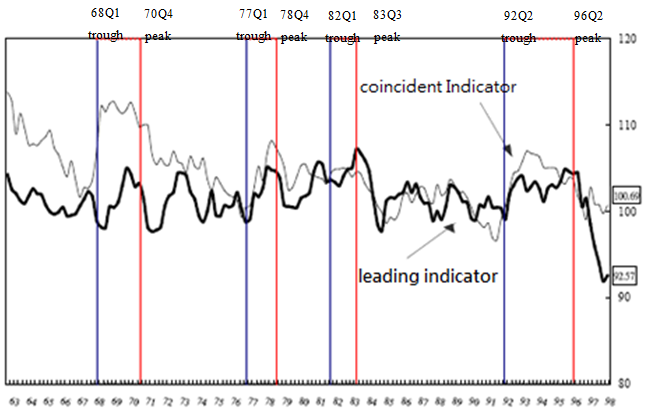
Figure-4. Real estate business cycle leading and coincident indicator composite index trends

Source: Architecture and Building Research Institute, Ministry of the Interior, Taiwan Real Estate Research Center, National Chengchi University (Quarterly report of Taiwan’s real estate business cycle trends, December 2009)

In order to observe the changes of the real estate business cycle leading indicator and HMM model forecasting capabilities by following the practice of the 4-step out-of-sample forecasting method, this study uses the average change rate of the features of the state optimal path to estimate the real estate business cycle leading indicator. The model estimated trend forecasting is as shown in Figure 5. Between 1972 Q3 and 1974 Q4, the model estimation has apparent lagging trends. The trends of the upward and downward fluctuations of the model forecasting are in the same direction with those released by the Taiwan Real Estate Research Center. Wherein, there are five decreasing forecasting values, which are consistent with the real estate leading indicators released by Taiwan Real Estate Research Center, in particular, those for the period of 1971 Q2~Q4 and the period of 2008 Q1~Q4. As far as the business cycle fluctuations deepness is concerned, the HMM-estimated leading indicator is deeper than the real indicator in the state of recession. Changes in forecasting average fluctuations suggest significant differences. These differences are caused by the different number of states.

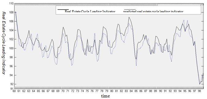
Figure-5. predicted trends of real estate business cycle leading indicator

Source: Compiled by this study.

5. CONCLUSION

Based on the time series data of the real estate business cycle composite leading indicator jointly compiled and regularly released by the Architecture and Building Research Institute, as well as the Taiwan Real Estate Research Center of National Chengchi University, this paper uses the HMM to capture the optimal path of state transition to observe the trends of fluctuations of out-of-sample data. Regarding the identification and application of the economic cycle leading indicators and HMM model in the trends of business cycle fluctuations, the results confirm that trends of the real estate business cycle fluctuations are asymmetric and that the average duration of recession periods is longer than that of expansion periods.

By overcoming the unobservable limitation of using the Markov-switching model to capture state series setting, this study applies the univariate discrete HMM model and feature extraction method to extract signals from the unobservable state to increase data simulation. Overall, the in-state observation value probability is consistent with the market fluctuations that the HMM model extracts for the in-state observation values to observe the unobservable state of the Markov-switching model. In terms of the out-of-sample 4-step-ahead forecasts, except for the sections of the fluctuations of structural change, the results of the mean absolute error rate of the estimation accuracy suggest that the average accuracy of using the HMM model to forecast 4-step out-of-sample state is up to 55.41%. This indicates that the proposed model is advantageous in model estimation.

However, the proposed model has not considered the differences caused by the fluctuation trend path estimation due to structural change. Therefore, it cannot effectively master the fluctuation path of total samples in the current term. Previous studies have suggested that the leading indicator is not only useful for setting and selection but can also serve as the leading reminder of macroeconomic phenomena. Therefore, future studies can use the improved dual-layer built-in HMM measurement models based on the leading indicator series compiled by the Taiwan Real Estate Research Center, such as the multivariate Markov vector auto-regression model for describing the common fluctuation characteristics between series (Krolzig, 1997) the switching probability time-varying Markov-switching model (Peersman and Smets, 2001) the duration dependent Markov-switching model of switching probability with duration dependent characteristics (Pelagatti, 2001) or the continuous hidden Markov-switching model, to further reduce forecasting error.

Note

Note 1: The leading indicator composite index is compiled by the Taiwan Real Estate Research Center, College of Social Sciences, National Chengchi University, at the delegation of Construction and Planning Agency, Ministry of the Interior. Starting with the first quarter of 1971, it initially consisted of relevant macroeconomics indicators including GDP, monetary supply, and CPI. In 1981 and 1989, indicators relating to the real estate industry and the construction stock index as well as the construction credit balance change were used to form the current real estate business cycle leading composite index.

Note 2: The state transition model is a non-linear model. It can be divided into two types by the state transition observation. If the model’s state transition process is determined by the observable variables, it is known as the threshold model, in which case state change is determined by whether the observable variable is above the threshold value. If it is above threshold value, the state transition occurs. For another type of the model, the state transition process is determined by the unobservable variables. Therefore, the model should define the state transition process. The Markov switching model is such a model. The Markov switching model considers that data come from different parent matrices. By setting a group of self-regression equations and using a Markov chain to understand the inter-state switching process, the current term state will be subject to the influence of the previous state, so that the data of various periods will be continuous and relevant. The probability theory can be applied to estimate the non-linear shifting of state transitions.

Note 3: In the HMM model, there are a number of patterns of hidden in-state observation output sample spaces and probability distributions such as univariate discrete observations, continuous observations, and mixed continuous observations. This paper sets the output observations as type of univariate discrete data distribution.

Note 4: There are a number of general patterns for the HMM model. The main change is that inter-state switching probability can switch in between states without limitation. Second, the pattern of the in-state observable value can be univariate discrete data, univariate continuous data, multivariate discrete data, or multivariate continuous data. To summarize, the two assumptions of this study should be satisfied, that is, in-state observation value o_m and state q_t are mutually dependent and mutually independent with o_m. The first-order Markov assumption and the current term switching probability are subject to the influence of the current term and previous term switching probability only.

Note 5: The term “stationary series” means that the statistical characteristics of the time series data generation process, including average, variance, and covariance, should be limited constants. It expects the time series variable’s important statistical characteristics including average, variance… to be non-time-varying to facilitate statistical inference and parameter estimation. On the other hand, if it is misused, it can easily lead to estimation bias. The most well-known example of such bias is proposed by Granger and Newbold (1974) when they note that spurious regression often occurs in between non-stationary variables.

Note 6: In Taiwan’s real estate business cycle trend quarterly reports, the scores are given in terms of changes in the indicators. The real estate business cycle trend signals are categorized into five lights, specifically, red, yellow-red, green, yellow-blue, and blue lights, to represent business indicators of ranging from a significant increase to a significant decrease including overheated business, business boom, business stability, poor business, and business recession.

Note 7: The term “rolling window” refers to the sampling method of a given sample length and sampling period range shifting by term.

Note 8: The estimation of the business duration period is determined by the computation of inter-state switching probability, that is, represent the average duration periods of the market recession, market of no change, and market expansion.

Note 9: The term “business cycle asymmetry” refers to the inconsistency in the durations of expansion and recession periods in business cycles. Sichel (1993) proposed two features relating to business cycle asymmetric fluctuations: deepness and steepness. In that study, deepness is described as the inconsistency in the distance from the trend values in the case of valley and peak of the business cycle in fluctuations. In addition, steepness is mainly used to describe the inconsistency in the slope of the valley and peak movements in the business cycle, that is, the speeds at which rebounds from the peak and the valley occur are not the same.

Note 10: According to the data released by the Taiwan Real Estate Research Center, the current average expansion period lasts 9 seasons and the average recession period lasts 24 seasons, indicating an apparent asymmetry of longer business recessions than expansions.

Funding: This study received no specific financial support.

Competing Interests: The authors declare that they have no competing interests.

Contributors/Acknowledgement: All authors contributed equally to the conception and design of the study.

REFERENCES

Arsenault, M., J. Clayton and L. Peng, 2013. Mortgage fund flows, capital appreciation, and real estate cycles. Journal of Real Estate Finance and Economics, 47(2): 243-265.

Barras, R., 2005. A building cycle model for an imperfect world. Journal of Property Research, 22(2): 63-96.

Baum, A., 2001. Evidence of cycles in European commercial real estate markets and some hypotheses. A global perspective on real estate cycles. US: Springer. pp: 103-115.

Baum, L.E. and T. Petrie, 1966. Statistical inference for probabilistic functions of finite state Markov chains. Annals of Mathematical Statistics, 37(6): 1554-1563.

Bouchaffra, D. and J. Tan, 2004. Introduction to the concept of structural HMM: Application to mining customer's preferences in automative design. 17th International Conference on Pattern Recognition. IEEE. pp: 493.

Cai, J., 1994. A Markov model of switching-regime ARCH. Journal of Business & Economic Statistics, 12(3): 309-316.

Chen, M.C., 2003. Time-series properties and modelling of house prices in Taipei area: An application of the structural time-series model. Journal of Housing Studies, 12(2): 69-90.

Chen, S.W., 2006. An analysis of the effect of output volatility on turning points identification: International evidence. Journal of Social Sciences and Philosophy, 18(1): 37-76.

Clayton, J., 1996. Market fundamentals, risk and the Canadian property cycle: Implications for property valuation and investment decisions. Journal of Real Estate Research, 12(3): 347–367.

Cruz, M., 2005. A three-regime business cycle model for an emerging economy. Applied Economics Letters, 12(7): 399-402.

Edelstein, R.H. and D. Tsang, 2007. Dynamic residential housing cycles analysis. Journal of Real Estate Finance and Economics, 35(3): 295-313.

Goetzmann, W. and S. Wachter, 2000. The global real estate crash: Evidence from an international database, New York University Stern School of Business Salomon Center Publications, Real Estate Cycles, Editor, Stephen J. Brown and Crocker Liu.

Gordon, J., P. Mosbaugh and T. Canter, 1996. Integrating regional economic indicators with the real estate cycle. Journal of Real Estate Research, 12(3): 469-501.

Granger, C.W.J. and P. Newbold, 1974. Spurious regressions in econometrics. Journal of Econometrics, 2(2): 111-120.

Gray, S.F., 1996. Modeling the conditional distribution of interest rates as a regimeswitching process. Journal of Financial Economics, 42(1): 27-62.

Gregoir, S. and F. Lenglart, 2000. Measuring the probability of a business cycle turning point by using a multivariate qualitative hidden Markov model. Journal of Forecasting, 19(2): 81-102.

Grenadier, R., 1995. Local and national determinants of office vacancies. Journal of Urban Economics, 37(1): 57-71.

Hamilton, J.D., 1989. A new approach to the economic analysis of nonstationary time series and the business cycle. Econometrica, 57(2): 357-384.

Hamilton, J.D. and R. Susmel, 1994. Autoregressive conditional heteroscedasticity and changes in regime. Journal of Econometrics, 64(1-2): 307-333.

Hassan, M.R. and B. Nath, 2005. Stock market forecasting using hidden markov model: A new approach. Proceeding of the 5th International Confernece on Intelligent Systems Design and Applications. pp: 8-10.

Huang, M.C., 2013. The role of people’s expectation in the recent US housing boom and bust. Journal of Real Estate Finance and Economics, 46(3): 452-479.

Huang, X., A. Alex and H.W. Hom, 2001. Spoken language processing: A guide to theory, algorithm, and system development. New Jersey: Prentice-Hall Press.

Kan, K., S.K.S. Kwong and C.K.Y. Leung, 2004. The dynamics and volatility of commercial and residential property prices: Theory and evidence. Journal of Regional Science, 44(1): 95–123.

Korolkiewicz, M.W. and R.J. Elliott, 2008. A hidden Markov model of credit quality. Journal of Economic Dynamics and Control, 32(12): 3807-3819.

Koskinen, L. and L.E. Öller, 2004. A classifying procedure for signalling turning points. Journal of Forecasting, 23(3): 197-214.

Krolzig, H.M., 1997. Markov-switching vector autoregressions: Modelling, statistical inference and application to business cycle analysis. Berlin: Springer-Verlag, Lecture Notes in Economics and Mathematical Systems, 454.

Krystalogianni, A., G. Matysiak and S. Tsolacos, 2004. Forecasting UK commercial real estate cycle phases with leading indicators: A probit approach. Applied Economics, 36(20): 2347-2356.

Lee, C.C., C.M. Liang and H.J. Chou, 2009. Identifying turning points of real estate cycles in Taiwan. Journal of Real Estate Portfolio Management, 15(1): 75-85.

Leng, C.P. and S.C. Wang, 2014. Hidden Markov model for predicting the turning points of GDP fluctuation. International Conference on Future Computer and Communication Engineering.

Leung, C., 2007. Equilibrium correlations of asset price and return. Journal of Real Estate Finance and Economics, 34(2): 233–256.

Liu, H., 2010. Dynamic portfolio choice under ambiguity and regime switching mean returns. Journal of Economic Dynamics and Control, 35(4): 623-640.

Mueller, G.R., 1999. Real estate rental growth rates at different points in the physical market cycle. Journal of Real Estate Research, 18(1): 131-150.

Netzer, O., J.M. Lattin and V. Sirinvasan, 2008. A hidden Markov model of customer relationship dynamics. Marketing Science, 27(2): 185-204.

Oguz, H.T. and F.S. Gurgen, 2008. Credit card analysis using hidden Markov model. 23rd International Symposium on Computer and Information Sciences. Istanbul: IEEE.

Peersman, G. and F. Smets, 2001. Are the effects of monetary policy in the Euro area greater in recessions than in booms! European Central Bank, Working Paper, No. 52.

Pelagatti, M., 2001. Gibbs sampling for a duration dependent Markov switching model with an application to the U.S. business cycle. Working Paper. Quaderno di Dipartmento QD2001/2 (March), Dipartimento di Statistica, Universita degli Studi di Milano Bicocca.

Peng, C.W., C.C. Lin and Y.T. Yang, 2004. An analysis of structural changes in housing prices: Cases of Taipei City and Taipei. Journal of Taiwan Land Research, 7(2): 27-46.

Pritchett, C.P., 1984. Forecasting the impact of real estate cycles on investment. Real Estate Review, 13(4): 85–89.

Rau, H.H., H.W. Lin and M.Y. Li, 2001. Examining Taiwan’s business cycle via two-period MS models. Academia Economic Papers, 29(3): 297-319.

Roamn, D., G. Mitra and N. Spagnolo, 2010. Hidden Markov models for financial optimization problems. Journal of Management Mathematics, 21(2): 111-129.

Roulac, S.E., 1996. Real estate market cycles, transformation forces and structural change. Journal of Real Estate Portfolio Management, 2(1): 1-17.

Scott, P. and G. Judge, 2000. Cycles and steps in British commercial property values. Applied Economics, 32(10): 1287-1297.

Sepideh, S. and A. Aaghaie, 2011. Introducing busy customer Portfolio using hidden Markov model. Iranian Journal of Management Studies, 4(2): 99-119.

Shen, H. and J. Zhao, 2006. Classification customer loyalty based on hidden Markov model. International Journal of Internet and Enterprise Management, 4(1): 57-64.

Sichel, D.E., 1993. Business cycle asymmetry: A deeper look. Economic Inquiry, 31(2): 224-236.

Tvede, L., M.H. Hsiao and Y. Chen, 2008. Why business cycles-history, theory and investment practice. Taipei: Wealth Press.

Wu, F., I.H. Chiu and J.R. Lin, 2005. Prediction of the intention of purchase of the user surfing on the web using hidden Markov model. International Conference on Services Systems and Services Management. IEEE. pp: 387.

Wu, Y.L., 2009. Studies on the predicting power of leading indicator of Taiwan's real estate cycle - hidden Markov model analysis. Master Thesis, National Pingtung Institute of Commerce.

Zhu, Y. and J. Cheng, 2013. Using hidden Markov model to detect macro-economic risk level. Review of Integrative Business and Economics Research, 2(1): 238-249.

Views and opinions expressed in this article are the views and opinions of the author(s), Asian Economic and Financial Review shall not be responsible or answerable for any loss, damage or liability etc. caused in relation to/arising out of the use of the content.