ENERGY CONSUMPTION IS A DETERMINANT OF ECONOMIC GROWTH IN BRICS COUNTRIES OR NOT?

Tayfur BAYAT¹ --- Sebnem TAS² ---Izzet TASAR³⁺

¹Associate Professor, Inonu University, Faculty of Business Administration and Economics, Department of Economics, Malatya, Turkey
² Research Assistant, Firat University, Faculty of Business Administration and Economics, Department of Economics, Elazig, Turkey
³Assistant Professor, Firat University, Faculty of Business Administration and Economics, Department of Economics, Elazig, Turkey

Keywords:Energy consumption, Conservation Hypothesis, Feedback Hypothesis, Economic growth, Panel data, BRICS.

JEL Classification:Q43, F43, C23.

ARTICLE HISTORY: Received:25 April 2017 Revised:31 May 2017 Accepted:13 June 2017 Published:5 July 2017

Contribution/ Originality:: This study contributes in the existing literature by the countries selected. BRICS countries are a good example in terms of economic growth in our decade. In addition, the energy consumption is another level compared to the rest of the world in those countries. One of the basic questions, the link between energy consumption and the economic growth is responded in the article.

1. INTRODUCTION

The relationship between energy consumption and economic growth determines the nature of energy politics as well as growth policies. The optimal energy policy for the country can also be determined if the relationship between energy consumption and economic growth is correctly determined, since CO2 emissions associated with energy consumption triggers global warming, which is considered to have adverse effects on prosperity of future generations. If energy consumption at this point provides economic growth in a country, reducing energy consumption in order to prevent its negative impact on the environment will be an appropriate policy (Huang et al., 2008).

The relationship between energy consumption and economic growth is defined by four hypotheses in the literature. Growth hypothesis is defined as the one-way causality towards from energy consumption to growth. On the other hand conservation hypothesis is the one-way causality from growth to energy consumption. In the presence of the growth hypothesis, it plays a key role in promoting energy economic activity, and a reduction in energy consumption leads to a decline in economic growth (Asafu-Adjaye, 2000). In that parallel, the policy applied should not increase the energy prices and therefore the energy consumption cuts. In the conservation hypothesis; Energy conservation policies based on energy saving can be implemented without hindering economic growth, since there is no energy dependence for economic growth (Bulut et al., 2014). The two-way causality between economic growth and energy consumption is called the feedback hypothesis, and in such a case, the change in any of the variables will affect the other (Ahmad et al., 2016). Finally, in the neutrality hypothesis argues that there is no significant relationship between energy consumption and economic growth. In such a case, it would be appropriate to monitor policies focused on conservation of the ecological system by limiting the country's energy use and increasing energy efficiency (Bulut et al., 2014).

This study examines whether energy consumption in BRICS countries is a determinant of economic growth. BRIC that is (Brazil, Russia, India, China), the initials of Brazil, Russia, India and China, was first used in conjunction with the research report, Building Better Global Economic BRICs, prepared by Goldman Sachs chairman (O’neil, 2011). In addition to being the fastest-growing "emerging markets" in the world, the four countries in question have many common characteristics such as having large surface area, overcrowding and rapid and steady growth in recent years. These countries, which encompass 25% of the world's surface area and 40% of the world's population, are rapidly developing as global market economies, and with this rising momentum they will be able to leave behind G7 countries (Canada, France, Germany, Italy, Japan, USA) (Narin and Kutluay, 2013). However, in recent years it was argued that new countries, defined as emerging markets should be included in the BRIC and BRIC after the inclusion of South Africa (South Africa) in April 2011, Expanded to BRICS (Kaya and Yalçinkaya, 2016).

Following the introduction, the literature review will considered in the second part, the methodology in the third part, the empirical results in the fourth part and finally the conclusion and the policy proposal in the last part.

2. LITERATURE REVIEW

The number of studies examining the relationship between energy consumption and economic growth has increased rapidly over the last three decades. Along with the surplus of studies in the literature, it is generally observed that there is a contradiction between the findings. The reasons for this outbreak are the specific characteristics of the countries covered, the employed testing techniques and approaches, and the variations in the data set and periods. There are three different analysis for American economy; Kraft and Kraft (1978) in their empirical results support conservation hypothesis, Stern (2000) supports growth hypothesis, and Akarca and Long (1980) supports hypothesis of neutrality. This diversity in the results obtained can be attributed to the fact that the data belong to different time periods, and that different test techniques and approaches are used. Moon and Sonn (1996) investigated an economic growth model in South Korea based on annual data from 1968 to 1989. At the beginning, they pointed out that there was an inverse U-shaped non-linear relationship between economic growth and energy consumption, which increased with efficient energy spending but then decreased. Glosure and Lee (1997) examined the relationship between energy consumption and gross domestic product for South Korea and Singapore using the Granger causality test based on the vector auto regression model, the co-integration and error correction model. According to the results of the co-integration and error correction model, they obtained two-way causality between income and energy in both countries. Another consequence of not working is that there is no causality relationship in South Korea, but in Singapore it is determined that Granger causality from energy to gross domestic product. Asafu-Adjaye (2000) investigated the relationship between energy consumption and income. Co-integration and error correction model are employed in the analysis. Tests cover India, Indonesia, Philippines and Thailand. According to the empirical results, there is a one-way Granger causality from the energy consumption to GDP in India and Indonesia in the short term and bi-directional Granger causality between energy consumption and income in Thailand and the Philippines. Paul and Bhattacharya (2004) suggest bi-directional causality for India's energy consumption and economic growth according to co-integration and Granger causality tests for the period 1950-1996. Lee (2005) examined the relationship between energy consumption and economic growth for 18 developing countries between 1975-2001. Lee (2005) used panel root test, heterogeneous panel co-integration and panel-based error correction. In the short and long term, causality from energy consumption to economic growth.is supported. Lee and Chang (2007a) analyzed the relationship between energy consumption and economic growth using a dynamic panel data approach for 18 developing and 22 developed countries. Economic growth in developing countries leads to energy consumption, while in developed countries, bi-directional hypothesis is supported. Lee and Chang (2007b) used total energy consumption as a threshold variable to determine the existence of a non-linear relationship in single and two sector growth models. They stressed that there was an inverse relationship between energy consumption and economic growth in Taiwan between 1955-2003. Huang et al. (2008) in a panel data analysis for 82 countries, countries were divided into low income group, lower middle income group, upper middle income group and high income group as defined by the world bank. According to the findings of the study; In the lower and upper middle income countries, economic growth positively affects energy consumption. In the high income group, there is no relationship between economic growth and energy consumption in the negative direction and finaly in the low income group there is no significant relation among variables. Payne (2009) found no relationship between variables renewable and non-renewable energy consumption in the US and the real gross domestic product, they employed Toda-Yamamoto causality test results. Odhiambo (2009) has added the employment rate as an intermittent variant of two variable models of electricity consumption and economic growth, and the simple bit has created three variable causality disturbances and they approved the validity of the Bi-directional causality between electricity consumption and economic growth.

Cowan et al. (2014) examined electricity consumption, economic growth and CO2 emissions in BRICS countries using panel causality analysis. Bi-directional causality between electricity consumption and economic growth in Russia is valid according to the test results. Causality from economic growth to energy consumption in South Africa, and no valid causality in Brazil, China and India. Hu et al. (2015) tested the relationship between energy consumption and economic growth using panel data from China's 37 industrial sectors, from 1998 to 2010. The panel vector error correction model is employed in the analysis and one-way causality in the short-term from economic growth to energy consumption is approved. Secondly one-way causality in the long-term from energy consumption to economic growth was found. Ahmad et al. (2016) found a cointegration relationship in their analysis among CO2 emissions per capita, real GDP per capita and energy consumption per capita in their analysis for India in the period 1971-2014.

3. METHODOLOGY

3.1. Cross-Section Dependency and Homogeneity

In the model above, CD has zero mean for the fixed T and N. The dynamic model includes multiple breaks in slope coefficients and/or error variances. In the model dependent and independent variables are time-invariant and have symmetric distributions. Because of the fact that Pair-wise correlations does not have zero mean distribution (Pesaran et al., 2008) calculated new bias-adjusted LM test statistics for large panels;

3.2. Cross-Sectional Augmented Dickey–Fuller (CADF) Unit Root Test

Pesaran (2007) modifies the ADF regressions by changing the cross-section averages of lagged levels and first-differences of the individual series. Then, the cross-sectional augmented Dickey–Fuller (CADF) regression is as follows;

3.3. Im et al. (2005) Unit Root Test with Structural Break

3.4. Panel Co-Integration and Causality

The critical values are calculated via bootstrap method in order to consider the cross section dependency. Null hypothesis rejects the co-integration. Emirmahmutoğlu and Kose (2011) gains causality for each “i” by implementing bootstrap method on Fisher test statistics. First the optimal lag length for each “i” is calculated according to information criteria by employing unit root test (dmaxi);

4. AMPIRICAL RESULTS

Energy consumption (EC) and Gross Domestic Product Growth Rate (GDP) variables are included in the analysis. As mentioned before Brazil, Russia, India, China and South Africa countries are considered for the period from 1990 to 2013. The data for is obtained from World Bank Database. All data is in log form for the analysis.

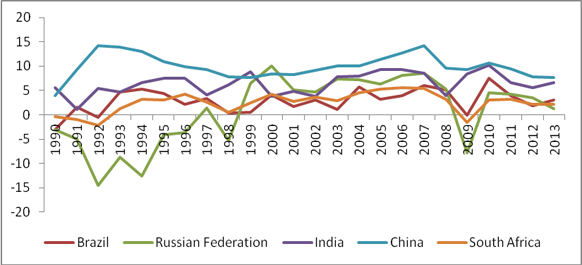
Graph-1. Economical Growth Rate for Countries

Source: World Bank Database, own Calculation

When the growth performance of BRICS countries between 1990 and 2013 is considered, there is a remarkable country with the highest growth rate, that is China. Following the steady growth rate of China, which entered a rapid upward trend at the beginning of 1990s and an average of around 11% each year. This result is not a surprise, it is a result of the government policies that focused on the economic development as its main policy after 1978. Main stream in this policy change was a series of changes in agriculture, foreign economic relations and public administration. In particular, the open-door policy, which is an important component of China's reform, initially created free-zones near Hong-Kong and Taiwan then those are followed by other free zones. Also other main policies such as foreign investment liberalization and tax reduction resulted China to be the biggest manufacturing industry exporter. In more recent times, China's industrial policy switched from low cost production to build and develop high added-value, technology-intensive industries. According Graph 1, it appears that China has survived the 2008 crisis with only a slight decrease in the growth rate, without a steady economic recovery (Oz, 2010). Graph shows that India follows China with a growth rate does not go below %5. India shows a more volatile structure compared to China in the mentioned period. Increase in the exports after liberalized foreign trade policy supported success of India. India became an important software supplier in the world, that depends on the government investments aimed to increase educated human capital. That also resulted a young generation that speaks English in that parallel it was a chance to host the call centers of multinational companies operating in fields such as banking and insurance. India with that improvments got the advanced financial system and science and technology infrastructure. India also did not live the 2008 crieses in deed according (Oz, 2010). Especially after 1991, the disintegration of SSCB, Russia abandoned its long-standing central planning tradition and tried to adapt to the free market economy through comprehensive reform programs, especially in the area of ​​privatization. Russia is also concentrating on energy exports because of its natural resources (Akbulak, 2008). The fast adaptaion period resulted a volatile economy till 1997. The growth rate is mostly negative in that period. Economy had positive growth rate only after 1996, but that was not a start of the growthi just after 1 year the South East Asia crises in 1997 resulted a demand shcok in energy sector and in Russian economy. Afterwards, 1998 Russia crises was not a surprise. The rises in the energy prices in the world economy resulted a positive trend in Russia economy till 2008. Russia was not lucky as China or India in 2008, truly Russia performed the worst performance in 2008 crises in BRICS. As it was in 1997, the contraction in the economy caused a decrease in energy demand and the prices fall down sharply. In Brazil, the liberalization process started in 1990 and it caused a rapid growth. The economy mainly specilazied in automotive industry. Privatization had an advantage to modernize the infrastructure, an growth was positive till 1998. Integrated world and the financial markets carried the crises in South East Asia to Brazil very quickly. The international investors, felt uncomfortable especially after 1994 that Brazil started to depriciate Real against USA dollars. Also the current account deficit was not trusted to be sustainable. Lastly, in 1998 Minas Gerais state rejected all debts and payments to the central government and bankruptsy was inevitable (Turan, 2011). After the crisis in 1998, the growth rate has dropped to zero. Following the devaluation in January 1999, a rapid recovery in the economy was a result of the reforms that implemented with the IMF agreement. Positive growth trends up to 2008, after the global financial crisis, demand and liquidity shrinkage around the world have reduced the amount of foreign capital entering the country and the growth rate decreased. The regulations on the credit market, the banking system and export incentive systems, the crisis has been passed quickly and a rapid growth started. The South African economy, dominated by rich mineral resources and arable land, mining and agriculture, has been transformed in recent years and the role of secondary sectors in the economy has begun to grow. The growth rate, which was negative started to be positive after 1992. The 1997 South East Asian crisis and 2008 world crises resulted negative growth in the economy, however, the immediate recovery policies aftermath of the crisis, recovered the economy.

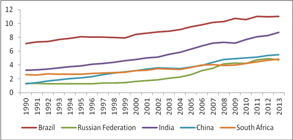
Graph-2. Energy Consumption

Source: World Bank Database, own Calculation

If the energy concumption of the BRICS countries considered, Brazil is on the top in Graph 2. After Brazil countries are ranked as follows; India, China, South Africa and Russia. Especially Brazil, India and China have an increasing trend on energy consumption. On the other hand, Soıth Africa is more stable and Russia has the upward trend after crises.

In panel data analysis to determine if each i is correlated to each other or not, cross section dependency is performed before unit root test. If there is no cross section dependency, the 1st Generation unit root tests are used and if the cross section dependency is exists, the 2nd Generation unit root tests are performed. Panel data analysis employs Pesaran (2004) CDLM, Breusch-Pagan CDLM1, and Pesaran (2004) CDLM2 tests to test cross section dependency. CDLM1 and CDLM2 are used if T> N, that is the time dimension is greater than the horizontal dimension. The CDLM test is used if N> T; that is the opposite case. In the cross section dependency tests, the null hypothesis is there is no cross section dependency and the alternative hypothesis argues the existence of cross section dependency.

Table-1. Cross Section Dependency Test

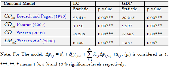
If the probability ratio is considered, the alternative hypothesis is accepted; there is cross section dependency. For all selected variables, cross-sectional augmented Dickey–Fuller (CADF) 2. Generation unit root test will be applied. Null hypothesis in CADF test support the existence of a unit root in the data, and the alternative is opposite. If the CADF statistic is smaller than the critical value, that mean the data belong to that country is stationary. Otherwise, if the opposite situation holds, the series are not stationary.

When the test statistics are compared with Pesaran (2007) critical values, the results offer the existence of unit root for China both in constant and constant and trend. For GDP growth variable, Russia, India and South Africa has unit root in constant, whereas only South Africa has unit root in both constant and constant and trend. Im et al. (2005) Unit root test that considers structural breaks offers the existence of unit root in alternative hypothesis. For the test results, if the test statistics is bigger than the critical value, the null hypothesis is rejected and alternative hypothesis is accepted.

Table-2. CADF Unit Root Test

		Constant		Constant and Trend
	Lags	CADF-stat	Lags	CADF-stat
EC
Brazil	3	-2.628	1	-1.959
Russia	3	-1.276	4	-2.465
India	4	-0.581		2	-1.51
China	4	-1.669		4	-4.630**
South Africa	1	-2.213		1	-2.164
Panel		-1.673			-2.545
GDP
Brazil	4	-2.672		4	-3.338
Russia	4	-3.343**		4	-3.277
India	2	-3.329*		2	-3.095
China	1	-2.853		1	-2.847
South Africa	4	-3.710**		4	-3.963**
Panel		-3.181***			-3.304

Notes: Maximum lag length is considered 4, and optimal lag lengths are determined according to Schwarz information criteria. Critical value for CADF test; for the constant model -4.11 (%1), -3.36 (%5) and -2.97 (%10) (Pesaran, 2007) table I(b), p:275); for the constant and trend model -4.67 (%1), -3.87 (%5) and -3.49 (%10) (Pesaran, 2007) table I(c), p:276).  Panel statistics critical value, for the constant model -2.57 (%1), -2.33 (%5) and -2.21 (%10) (Pesaran, 2007) table II(b), p:280); constant and trend model -3.10 (%1), -2.86 (%5) and -2.73 (%10) (Pesaran, 2007). Panel statistics are the arithmetical average of, CADF statistics.

Tablo-3. Im et al. (2005) Panel Unit Root Tests With Structural Break

	One break model
	Level shift model:			Level and trend shift model:
	Break in Constant			Break in constant and trend
GDP	Lag	LM-stat.	Break Time	Lag			Transformed	Break Time
							LM-stat.
Brazil	4	-5.158***	1998	4			-5.168***	2002
Russia	0	-4.567**	1999	0			-4.526**	1999
India	0	-4.674***	2003	0			-4.474**	2003
China	1	-2.681	2007	1			-2.686	1996
South Africa	0	-4.046**	2008	0			-5.707***	2007
Panel-LM		-7.956***					-6.329***
p-value		0					0
		Two breaks model
Brazil	0	-6.456***	1996-2007		0	-6.349***		1996-2008
Russia	0	-4.604**	1999-2007		0	-5.248**		1997-2008
India	0	-5.656***	2001-2011		0	-6.686***		1999-2004
China	1	-6.462***	2004-2009		1	-7.324***		2006-2011
South Africa	3	-5.831***	1996 2007		0	-7.411***		1999-2007
Panel-LM		-13.412***				-12.469***
p-value		0				0

	One break model
	Level shift model:			Level and trend shift model:
	Break in constant			Break in constant and trend
EC	Lag	LM-stat.	Break Time	Lag	Transformed	Break Time
					LM-stat.
Brazil	2	-2.882	1998	2	-3.106	1998
Russia	3	-2.655	1996	3	-3.022	2004
India	0	-2.862	1996	0	-2.857	1999
China	1	-3.804*	2011	1	-3.945*	2010
South Africa	0	-4.782***	2001	0	-4.782***	2001
Panel-LM		-5.070***			-3.014
p-value		0			0
		Two breaks model
Brazil	0	-4.882**	1996-2005	0	-6.072***	1999-2009
Russia	3	-11.967***	1999-2009	3	-7.990***	1999-2010
India	1	-7.593***	1996-2004	1	-7.275***	1996-2004
China	1	-7.556***	2002-2009	1	-9.036***	2002-2009
South Africa	0	-5.746***	1996-2001	0	-6.405***	2001-2005
Panel-LM		-19.375***			-15.407***
p-value		0			0

Notes:
Critical values for individual statistics for one break model:  -4.604 (1%); -3.950 (5%); -3.635 (10%)
Critical values for individual statistics for two breaks model:  -5.365 (1%); -4.661 (5%); -4.338 (10%)
Maximum lag length is considered 4 and optimal lag length are determined according to “t-stat significance” approach.
***, **, * figures donated 1 %, 5 % and 10 % respectively.

According to Im et al. (2005) test results in Table 3, break dates for Brazil is as follows: for GDP variable; in the constant model with one break 1998, in the constant with trend model 2002 are the break dates. On the other hand, for the same variable constant model with two break shows 1996 and 2008 and constant-trend model shows again 1996 and 2008. In general, Brazil lived both Russia and world crises deeply. As it is obvious, especially same group economies affect each other in the global markets. In Russia, for GDP variable; in the constant model with one break 1999, in the constant with trend model 2009 are the break dates. On the other hand, for the same variable constant model with two break shows 1999 and 2007 whereas constant-trend model shows 1997 and 2008. Break dates in Russian economy also point out economic crises. Test results for Indian economy are not consistent with Brazil and Russia, Brazil has its dynamics. For GDP variable; in the constant model with one break 2003, in the constant with trend model again 2003 are the break dates. On the other hand, for the same variable constant model with two break shows 2001 and 2011 and constant-trend model shows 1999 and 2004. Apart from the Russia crises, India did not affected even in world crises. In China, for the first two model with one break there is not a statistically significant break date. Two break models offers 2004 - 2009 and 2006-2011 for constant and constant with trend respectively. For South Africa; in the constant model with one break 2008, in the constant with trend model 2007 are the break dates. On the other hand, for the same variable constant model with two break shows 1996 and 2007 and constant-trend model shows 1999 and 2007. The end of Apartheid regime has a positive effect in the international trade. That is after 1994. World crises also influenced South African economy. For the other variable, energy consumption, (EC) the results are as follows: Only China and South Africa has significant break dates in 2011 and 2010 respectively. For the two break constant model, in Brazil 1996-2005, Russia 1999-2009, India 1996-2004, China 2002-2009 and finally South Africa 1996-2001. On the other hand, break dates in constant and trend model are; for Brazil 1999-2009, Russia 1999-2010, India 1996-2004, China 2002-2009 and South Africa 2001-2005. It is difficult say that two variables has the same reactions in the selected period. In general, GDP and EC are mostly have breaks in world crises.

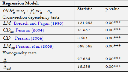
Table-4. Cross Section Dependency and Homogeneity Tests

Note: ***, **, * figures present 1 %, 5 % and 10 % levels respectively.

When the probability values are considered, the alternative hypothesis that argues the existence of both cross section dependency and heterogeneity is accepted. According to that test results, co-integration test that considers cross section dependency and heterogeneity will be employed.

Table-5. Panel Co-Integration Test Ignoring Structural Break

	Constant				Constant and Trend
	Statistic	Asymptotic	Bootstrap		Statistic	Asymptotic	Bootstrap
		p-value	p-value			p-value	p-value
Error Correction
Group_tau	-2.075	0.019**	0.179		-3.561	0.00***	0.086*
Group_alpha	-1.264	0.103	0.306		-2.563	0.00***	0.13
Panel_tau	-1.028	0.152	0.432		-6.109	0.00***	0.011**
Panel_alfa	-1.68	0.046	0.413		-7.519	0.00***	0.027**

Notes: Null hypothesis of the test ignores co-integration. Lag Length is considered as 1 in Error Correction Test. Bootstrap probability value is gained after 1.000 re-distribution. Asymptotic probability values are gained from standard normal distribution. ***, **, * show 1 %, 5 % and 10 % levels, respectively

According to test results, especially in the model with constant and trend, for both asymptotic and bootstrap values the alternative hypothesis is accepted; that supports the co-integrations among the variables.

Table-6. Emirmahmutoğlu and Kose (2011) Panel Causality

Country	Lag	GDP=>EC		EC=>GDP
		Wald	p-value	Wald	p-value
Brazil	3	7.61	0.054*	6.402	0.093*
Russia	1	5.04	0.024**	2.357	0.124
India	1	1.612	0.204	0.941	0.331
China	2	1.91	0.384	1.924	0.382
South Africa	1	0	0.998	0.775	0.378
Fisher		18.296	0.050*	14.974	0.132

Nots: ***, **, * presents 1 %, 5 % and 10 % significance levels respectively

Table 6 summarizes Emirmahmutoğlu and Kose (2011) panel causality test results. For Brazil, there is a significant bi-directional causality from economic growth to energy consumption. That causality relation holds in Russia only one way, that is from economic growth to energy consumption. Test results can not argue a significant causality relation among variables for countries India, China and South Africa. According to Huang et al. (2008) energy consumption will result in economic growth only if the value of energy efficiency and the value of emitted CO2 emissions are below a certain threshold in the declining state of cyclical fluctuations. However, in countries where CO2 emissions are above the threshold at the declining state of cyclical fluctuations such as China, India and South Africa economies, the situation will result as a negative externality created by environmental pollution by excessive energy consumption. That will not give the chance the economy to benefit from economic growth. Test results offers the validity of  that situation for 3 countries of BRIC out  of five. That offset effect will cause researchers to ignore the causality relation between energy consumption and economic growth. Cowan et al. (2014) also supports that explanation. In the research, they show high amounts of CO2  emission as a reason for the non-causality among energy consumption and economic growth. The high amounts of CO2  has different reasons for India and China. In China the production that increase in huge rates, where as in India the prevalence of coal in the industry results high rates of CO2  emissions. According to test results, Brazil performs different within BRICS group. Pao and Tsai (2011) explain that situation with the different emission and energy consumption profile of the country. More green energy in Brazil results a bi-directional significant causality from energy consumption to economic growth. Russia, according to Zhang (2011) should be considered as a producer of energy. Russia has lots of natural energy sources and with that specialty differs from other BRICS countries. The energy exports results in economic growth and that is also an increase in energy consumption. The most obvious example of this is the sharp decline in economic growth during the period of crisis caused by the transformation of the political system and the restructuring of the economy in 1991 and also the influence of the South East Asian crisis on Russia.

5. CONCLUSION AND POLICY IMPLICATIONS

Determining the determinants of economic growth will provide an important advantage in determining the growth policies for developing countries. Also the effect of energy consumption as a determinant of economic growth will be a serious tool for policy makers. In this study, the relationship between energy consumption and economic growth in the BRIC countries for the period 1990-2013 was analyzed by panel data method. Cross section dependency has been tested via Breusch and Pagan (1980); Pesaran (2004) and Pesaran (2007) Panel Unit Root Test approves the validity of cross section dependency. Westerlund (2007) panel co-integration test, which considers the cross section dependency, showed that variables move together in the long run. Emirmahmutoğlu and Kose (2011) panel causality test revealed the direction of causality relation for each country. According to this, the Brazilian economy has bi-directional causality and the Russian economy has causality from gross domestic product to economic growth. In China, India and South Africa, there is no significant linkage. Despite the similarities in the development performance of the BRICS countries, the associated differences in energy consumption and growth are due mainly to the energy efficiency of the energy used, the CO2 emission values ​​at the time of cyclical fluctuations, and the energy profiles. Huang et al. (2008) the energy consumption will cause economic consequences if the value of the energy used and the value of the emitted CO2 emissions are below a certain threshold value. The negative externality created by environmental pollution of excessive energy consumption in countries where the CO2 emission value is above the threshold will be heavier than it would be provided by economic growth. In the presence of such an offset effect, the existence of either a negative or a positive relationship between energy consumption and economic growth will not be discussed. Huang et al. (2008) supports the results of our study in their finding that there is no causality between energy consumption and economic growth in China, India and South Africa. This finding is called the neutrality hypothesis. In countries where this hypothesis is valid, energy consumption has no contribution to the growth so more conservative energy policies should be followed to minimize the negative impact of energy consumption on the environment. Within this scope, technologies that can increase efficiency in energy consumption can be utilized. Instead of energy consumption based on fossil fuels, measures can be taken to promote the use of clean and renewable energy such as solar energy, wind energy, nuclear energy and natural gas. In our study, the causality relation between economic growth and energy consumption for Russia is parallel to the Zhang (2011) analysis, and this relation is called the conservation hypothesis in the literature. In this respect, since there is no energy dependence on economic growth in Russia, so energy conservation-based energy policies can be implemented without hindering economic growth. Finally, test results approve the validity of feedback hypothesis for Brazilian economy, that is the causality relationship for Brazilian economy is bi-directional and also parallel to Pao and Tsai (2011) findings. The policies applied in energy or economy should be considered very carefully in such situation according to the fact that any change in economic growth or any change in energy consumption will affect the other.

Funding: This study received no specific financial support.

Competing Interests: The authors declare that they have no competing interests.

Contributors/Acknowledgement: All authors contributed equally to the conception and design of the study.

REFERENCES

Ahmad, A., Y. Zhao, M. Shahbaz, S. Bano, Z. Zhang, S. Wang and Y. Liu, 2016. Carbon emissions, energy consumption and economic growth: An aggregate and disaggregate analysis of the Indian economy. Energy Policy, 96: 131-143.View at Google Scholar | View at Publisher

Akarca, A.T. and T.V. Long, 1980. Relationship between energy and GNP: A reexamination. Journal of Energy and Development United States, 5(2): 326-331.View at Google Scholar 

Akbulak, S., 2008. BRIC’s ülkeleri ile Güney Kore ekonomilerine ve sermaye piyasalarına ilişkin temel göstergeler ve kısa değerlendirmeler, Sermaye Piyasası Kurulu Araştırma Raporu.

Asafu-Adjaye, J., 2000. The relationship between energy consumption, energy prices and economic growth: Time series evidence from Asian developing countries. Energy Economics, 22(6): 615-625. View at Google Scholar | View at Publisher

Breusch, T. and A. Pagan, 1980. The lagrange multiplier test and its application to model specification in econometrics. Review of Economic Studies, 47(1): 239–253. View at Google Scholar | View at Publisher

Bulut, C., D.D.F. Hasanov and E. Süleymanov, 2014. Enerji Kullanımı ve ekonomik büyüme ilişkilerinin teori ve ekonomi politikaları açısından değerlendirilmesi. Küreselleşme sürecinde Kafkaslar ve orta asya IV. Uluslararası kongresi, 2-4 Mayıs 2014.

Cowan, W.N., T. Chang, R. Inglesi-Lotz and R. Gupta, 2014. The nexus of electricity consumption, economic growth and CO 2 emissions in the BRICS countries. Energy Policy, 66: 359-368.View at Google Scholar | View at Publisher

Emirmahmutoğlu, F. and N. Kose, 2011. Testing for Granger causality in heterogeneous mixed panels. Economic Modelling, 28(3): 870–876. View at Google Scholar | View at Publisher

Glosure, Y.U. and A.R. Lee, 1997. Cointegration, error–correction, and the relationship between GDP and electricity: The case of South Korea and Singapore. Resource and Energy Economics, 20(1): 17–25.View at Google Scholar | View at Publisher

Hu, Y., D. Guo, M. Wang, X. Zhang and S. Wang, 2015. The relationship between energy consumption and economic growth: Evidence from China’s industrial sectors. Energies, 8(9): 9392-9406. View at Google Scholar | View at Publisher

Huang, B.N., M.J. Hwang and C.W. Yang, 2008. Does more energy consumption bolster economic growth? An application of the nonlinear threshold regression model. Energy Policy, 36(2): 755-767. View at Google Scholar | View at Publisher

Im, K.S., J. Lee and M. Tieslau, 2005. Panel LM unit-root tests with level shifts. Oxford Bulletin of Economics and Statistics, 67(3): 393-419. View at Google Scholar | View at Publisher

Kaya, V. and Ö. Yalçinkaya, 2016. İmalat sanayinin gelişimi, ekonomik büyüme ve cari açık ilişkisi: BRİCS ve seçilmiş yükselen piyasa ekonomileri (1992-2012). Atatürk Üniversitesi İktisadi ve İdari Bilimler Dergisi, 30(1): 91-119. View at Google Scholar 

Kraft, J. and A. Kraft, 1978. Relationship between energy and GNP. Review of Economic Studies United States, 3(2): 401-403.

Lee, C.C., 2005. Energy consumption and GDP in developing countries: A cointegrated panel analysis. Energy Economics, 27(3): 415–427.View at Google Scholar | View at Publisher

Lee, C.C. and C.P. Chang, 2007a. Energy consumption and GDP revisited: A panel analysis of developed and developing countries. Energy Economics, 29(6): 1206–1223.

Lee, C.C. and C.P. Chang, 2007b. The impact of energy consumption on economic growth: Evidence from linear and nonlinear models in Taiwan. Energy, 32(12): 2282–2294.

Lee, J. and M.C. Strazicich, 2003. Minimum lagrange multiplier unit root test with two structural breaks. Review of Economics and Statistics, 85(4): 1082-1089. View at Google Scholar | View at Publisher

Lee, J. and M.C. Strazicich, 2004. Minimum LM unit root test with one structural break. Manuscript, Department of Economics, Appalachian State University. pp: 1-16.

Moon, Y.S. and Y.H. Sonn, 1996. Productive energy consumption and economic growth: An endogenous growth model and its empirical application. Resource and Energy Economics, 18(2): 189-200. View at Google Scholar | View at Publisher

Narin, M. and D. Kutluay, 2013. Değişen Küresel Ekonomik Düzen: BRIC, 3G ve N-11 Ülkeleri. Ankara Sanayi Odası Yayın Organı, Ocak-Şubat.

O’neil, J., 2011. Building better global economic BRICs. Goldman Sachs Global Economics Paper No: 66.

Odhiambo, N.M., 2009. Electricity consumption and economic growth in South Africa: A trivariate causality test. Energy Economics, 31(5): 635-640. View at Google Scholar | View at Publisher

Oz, S., 2010. BRIC ülkelerinde ekonomik gelişmeler: Neden ayrı bir grup? TÜSİAD ve Koç Üniversitesi Ekonomik araştırma forumu, Politika Notu 10-15.

Pao, H.T. and C.M. Tsai, 2011. Modeling and forecasting the CO 2 emissions, energy consumption, and economic growth in Brazil. Energy, 36(5): 2450-2458. View at Google Scholar | View at Publisher

Paul, S. and R.N. Bhattacharya, 2004. Causality between energy consumption and economic growth in India: A note on conflicting results. Energy Economics, 26(6): 977-983.View at Google Scholar | View at Publisher

Payne, J.E., 2009. On the dynamics of energy consumption and output in the US. Applied Energy, 86(4): 575-577. View at Google Scholar | View at Publisher

Pesaran, H.M., 2004. General diagnostic tests for cross section dependence in panels. Working Paper No. 0435, University of Cambridge.

Pesaran, M.H., 2007. A simple panel unit root test in the presence of cross-section dependence. Journal of Applied Econometrics, 22(2): 265-312. View at Google Scholar | View at Publisher

Pesaran, M.H., A. Ullah and T. Yamagata, 2008. A bias-adjusted LM test of error cross section independence. Econometrics Journal, 11(1): 105–127. View at Google Scholar | View at Publisher

Pesaran, M.H. and T. Yamagata, 2008. Testing slope homogeneity in large panels. Journal of Econometrics, 142(1): 50-93.View at Google Scholar | View at Publisher

Stern, D.I., 2000. A multivariate cointegration analysis of the role of energy in the US macroeconomy. Energy Economics, 22(2): 267-283. View at Google Scholar | View at Publisher

Turan, Z., 2011. Dünyadaki ve Türkiye’deki Krizlerin Ortaya Çıkış Nedenleri ve Ekonomik Kalkınmaya Etkisi. Ömer Halisdemir Üniversitesi İktisadi ve İdari Bilimler Fakültesi Dergisi, 4(1): 56. View at Google Scholar 

Westerlund, J., 2007. Testing for error correction in panel data. Oxford Bulletin of Economics and Statistics, 69(6): 709-748. View at Google Scholar | View at Publisher

Zhang, Y.J., 2011. Interpreting the dynamic nexus between energy consumption and economic growth: Empirical evidence from Russia. Energy Policy, 39(5): 2265-2272.View at Google Scholar | View at Publisher

Views and opinions expressed in this article are the views and opinions of the author(s), Asian Economic and Financial Review shall not be responsible or answerable for any loss, damage or liability etc. caused in relation to/arising out of the use of the content.

---

Footnotes:

1. Please see Pesaran and Yamagata (2008). for test statistics.
2. See Im, Lee and Tieslau (2005). for test statistics.
3. See Emirmahmutoğlu and Kose (2011). for Boostrap test statistics.