BUSINESS CYCLES WITH PERIODIC SHOCKS IN A MULTI-COUNTRY AND MULTI-REGIONAL NEOCLASSICAL GROWTH MODEL

Wei-Bin Zhang¹

¹Ritsumeikan Asia Pacific University, Japan

Keywords: Business cycles.,Periodic shocks.,Propensity to save.,Propensity to consume housing.,Spatial agglomeration.,Regional.,National and global growth.,Regional amenity.

Article History: Received: 7 April 2017.,Revised: 2 May 2017.,Accepted: 29 May 2017.,Published: 19 June 2017

JEL Classification: R11, O18

Contribution/ Originality: This study contributes to the existing literature of nonlinear dynamic economics by generalizing the global economic growth model proposed by Zhang (2016). The study is one of very few studies that deal with business cycles of multi-country multi-region economic growth with microeconomic foundation.

1. INTRODUCTION

This paper generalizes the global economic growth model with any number of countries and each country with any number of regions recently proposed by Zhang (2016). Zhang’s model extends Uzawa’s two-sector growth model to a global economy for examining dynamic interactions between international trade, national and global growth, interregional migration, wealth accumulation and regional amenities. This study generalizes Zhang’s model by allowing all the time-independent parameters to be time-dependent. The generalization makes it possible to examine effects of any types of exogenous time-dependent shocks on the dynamic system cross regions and countries over time. We specially show how business cycles can be generated by different exogenous periodic shocks.

Zhang’s model provides insights into economic mechanisms of national spatial agglomeration and globalization which are taking place simultaneously in a well-connected world economy. There are only a few theoretical economic models which address these issues within a single comprehensive framework. The neoclassical economic growth model studies a global economy with multiple (any number of) countries and multiple (any number of) regions in each country. With regard to capital mobility and international and interregional trade, the model is based on the neoclassical growth trade model. The model is specially influenced by Oniki and Uzawa (1965) which studies trade patterns between two economies in the Heckscher-Ohlin modeling framework with fixed savings rates. Deardorff and Hanson (1978) propose a two country trade mode with different saving rates across countries. There are some other growth models with international trade (e.g., (Brecher et al., 2002; Nishimura and Shimomura, 2002; Bond et al., 2003; Ono and Shibata, 2005)). The study demonstrates the motion of global economies with multiple countries and multiple regions with the help of computer. Although spatial economists propose interregional dynamic models based on different factors of nonlinear dynamics (e.g., (Fujita et al., 1999; Forslid and Ottaviano, 2003)) most of the formal models in economic geography do not include capital/wealth accumulation as endogenous processes of industrialization and agglomeration. Tabuchi (2014) observes, “The scopes of most of the theoretical studies published thus far have been limited to two regions in order for researchers to reach meaningful analytical results. The two-region NEG models tend to demonstrate that spatial distribution is dispersed in the early period (high trade costs or low manufacturing share) and agglomerated in one of the two regions in the late period (low trade costs or high manufacturing share). However, it is no doubt that the two-region NEG models are too simple to describe the spatial distribution of economic activities in real-world economies. Since there are only two regions, their geographical locations are necessarily symmetric, and thus diverse spatial distributions cannot occur.” Not only does Zhang’s model include wealth accumulation as endogenous processes of the global growth, but also it takes account of environmental dynamics. This paper generalizes Zhang’s model by allowing all the time-independent parameters to be time-dependent. The paper is organized as follows. Section 2 defines the multi-country and multi-regional model with capital accumulation and economic structure. Section 3 identifies the differential equations which are applied to simulate the model of the global economy, plots the motion of the economic dynamics, demonstrates the existence of a unique equilibrium point, and proves the stability of the equilibrium point. Section 4 carries out comparative dynamic analysis with regard to exogenous perturbations in the total factor productivity of region’s industrial sectors, total factor productivity of region’s service sectors, propensity to save, regional amenity parameters, and propensity to consume housing. Section 5 concludes the study. The main analytical results of section 3 are proved in the appendix.

2. THE MULTI-COUNTRY AND MULTI-REGIONAL GROWTH MODEL

This study is to generalize Zhang’s dynamic multi-region model (Zhang, 2016). The generalization is carried out by allowing all the time-dependent variables to be time-dependent. This allows us to examine any exogenous change at any time. Zhang’s original model is influenced by the neoclassical trade theory with capital accumulation (Uzawa, 1961; Oniki and Uzawa, 1965; Brecher et al., 2002; Sorger, 2002). The model deals with a global economy with multiple national and multiple regional economies. The economy of each region is described as in the Uzawa two-sector model. Each region produces one capital good and one consumer good (services) and has one consumer good sector and capital good sector. The entire economic system produces only one capital good. The capital good can be used for capital accumulation and for consumption. Households own assets of the economy. All markets are perfectly competitive. Input factors are inelastically supplied and are fully utilized at every moment. Saving is undertaken only by households.

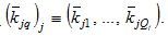
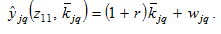
There are countries, indexed by Country consists of regions, indexed by The capital good is traded without any barriers. We measure prices in terms of the commodity and the price of the commodity is unity. The assumption of zero transportation cost of the commodity implies price equality for the commodity in the global economy. We denote wage and interest rates by and respectively, of region in country The interest rate is equalized throughout the global economy, i.e., Each country has a homogeneous population, denoted by This is no international migration. People in each country are free to choose their residential location. We assume that people work and reside in the same region. Each region has homogenous land which is only for residential use. 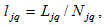Let and stand for the output levels of the capital good sector and service sector in region

2.1. The Capital Good Sectors

We denote the two productive factors, capital by and labor by at each point in time The production functions are

(1)

where and are parameters. The marginal conditions imply

(2)

where is the depreciation rate of physical capital in region

2.2. The Service Sectors

We denote the two productive factors, capital by and labor by at each point in time The production functions are

(3)

We use to represent region ’s service price. The marginal conditions imply

(4)

2.3. Behavior of Consumers

We assume absent landownership, which means that the income of land rent is spent outside the economic system. A possible reasoning for this is that as the land is owned by the government, people can rent the land in competitive market, and the government uses the income for military or other public purposes. Consumers choose lot size, consumption levels of services and the commodity, and saving. Let stand for the per household wealth in region Consumer obtains the current income from the interest payment and the wage payment as follows

(5)

The disposable income is the sum of the current come and the total value of wealth

(6)

The disposable income is used for saving and consumption. At each point in time, consumer distributes the total available budget among the lot size the saving the consumption of the capital good and consumption of services The budget constraint implies

(7)

where is region ’s land rent. The utility function is

(8)

in which and are the elasticities of utility of the consumer in country with regard to the lot size, capital good, services, and savings in region We call and the propensities to consume lot size, capital good, and services, and to hold wealth (save), respectively. In (8), is called region ’s amenity level. We specify as follows

(9)

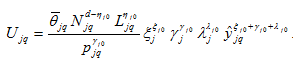
where and are parameters and is region ’s population. We don’t specify signs of as the population may have either positive or negative effects on regional attractiveness. Maximizing subject to the budget constraint yields

(10)

where

2.4. Wealth Accumulation

According to the definition of the wealth accumulation of the representative person is given by

(11)

The equation implies that the change in wealth is the saving minus the missaving.

2.5. Equalization of Utility Levels between Regions

As households are freely mobile between regions, the utility level of people in the same country should be equal, irrespective of in which region they live, i.e.

(12)

2.6. Capital and Wealth

We use and to denote the capital stocks employed by and the value of wealth owned by the population in region . We have

(13)

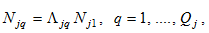
We use and to denote the capital stocks employed by and the value of wealth owned by country We have

(14)

The world capital stocks employed by the production sectors is equal to the total wealth owned by the households of all the countries. That is

(15)

2.7. Demand and Supply for Services

A region’s supply of services is consumed by the region

(16)

2.8. Full Employment of the Regional Labor

The labor force is fully employed in each region

(17)

2.9. Full Employment of the National Labor Force

The national labor force is fully used

(18)

2.10. The Regional Land Being Fully Used

Each region’s land is fully occupied for residential use

(19)

We thus built the model. The model is a special case of Zhang’s model (Zhang, 2016) in the sense that it is the same as Zhang’s model if all the parameters are constant. The model is general in the sense that it includes, for instance, the Solow growth model, the Uzawa two-sector growth model, and the Oniki-Uzawa trade.

3. SIMULATING THE MODEL

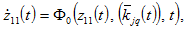
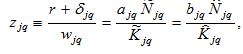
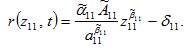
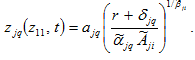
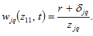
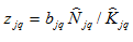
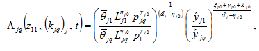
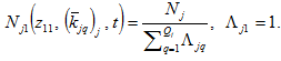
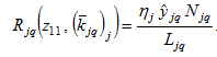
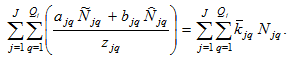
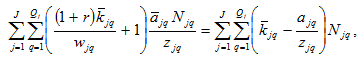
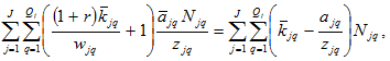
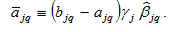
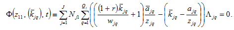
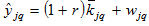
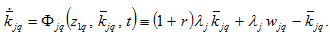
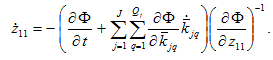
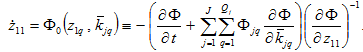
The world economy consists of any (finite) number of national economies. Although the dynamic system contains many time-dependent parameters, we provide a computational procedure for calculating all the variables at any point in time. In the appendix, we show that the dynamics of the global economy can be expressed as differential equations (in which one is actually algebra equation as shown in the appendix). First, we introduce a variable

Lemma

The motion of the global economy is given by the following differential equations with and as variables

(20)

where and are functions of and defined in the appendix. For any given positive values of and at any point in time, the other variables are uniquely determined by the following procedure: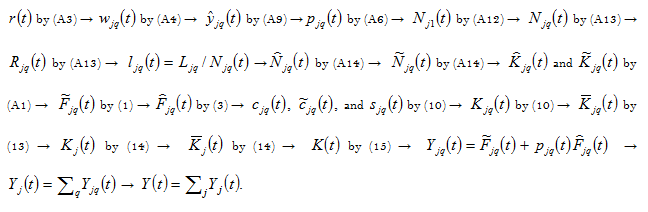

This result allows us to simulate the model with computer. As it is difficult to interpret the analytical results, to study properties of the system we simulate the model for a -country economy. The rest of this section follows Zhang (2016) in examining the motion of the system when all the parameters are constant. We specify parameter values as follows

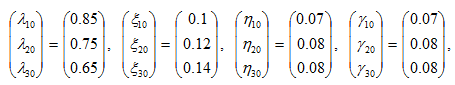
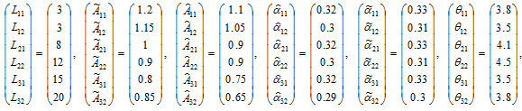
(21)

We specify the initial conditions as follows

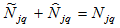
The motion of the variables is plotted in Figure 1.

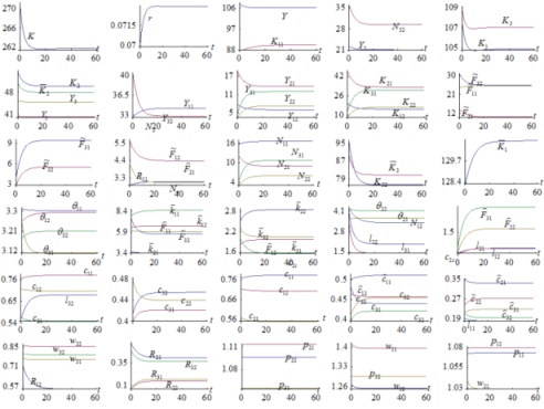
Figure-1. The Motion of the Economic System

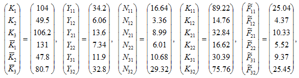
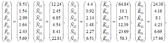
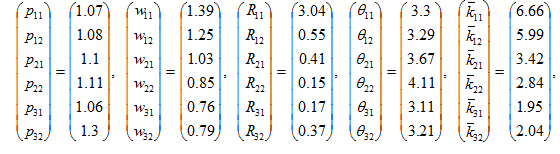
The simulation confirms that the system has a unique equilibrium. We list the equilibrium values in 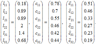(22)

(22)

It is straightforward to calculate the six eigenvalues of the differential equations evaluated at the equilibrium point as follow

The six eigenvalues are real and negative. The equilibrium is locally stable. This result is important as it guarantees the validity of comparative dynamic analysis in the next section.

4. COMPARATIVE DYNAMIC ANALYSIS

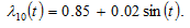
We simulated the motion of the global economy when all the parameters are constant as in (21). This study is interested in how the national and global economies behave when the system experiences time-dependent shocks. As the lemma in the previous section shows the computational procedure to calibrate the motion of all the variables with any type of exogenous shocks, it is straightforward to examine effects of change in any parameter. We consider the parameters in (21) as the long-term average values. We introduce different exogenous periodic perturbations around these long-term values. We use a variable to stand for the change rate of the variable, in percentage due to changes in a parameter.

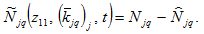
4.1. Perturbations in the Total Factor Productivity of Region (1, 1)’S Capital Good Sector

We first study the effects of the following perturbations in the total factor productivity of region ’s capital good sector

The simulation result is plotted in Figure 2. All the variables experience periodic changes with different amplitudes. The global income oscillates with greater amplitude than the global wealth. The wages of different parts of the global economy vary similarly. Country 1’s variables have great amplitudes in the perturbations.

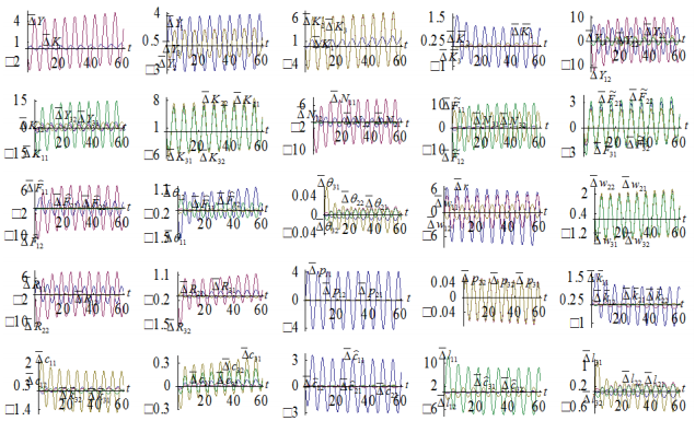
Figure-2. Perturbations in the Total Factor Productivity of a Capital Good Sector

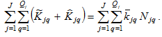
4.2. Perturbations in the Total Factor Productivity of Region (2 1)’S Service Sector

We now examine how the global and national economies react to the following periodic perturbations in the total factor productivity of region ’s service sector

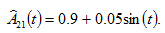
The simulation result is plotted in Figure 3. All the variables experience periodic. The global income and wealth fluctuate slightly with the technological fluctuation in the service sector. This is different from the impact of fluctuations in the capital sector’s total factor productivity. The wages of different parts of the global economy and rate of interest are slightly affected. Region ’s price and consumption levels of services fluctuate greatly, while the corresponding variables in the other regions change slightly. As services are locally consumed, the effects of technological changes tend to be reflected in the price and consumption of the local product.

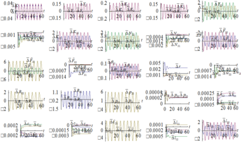
Figure-3. Perturbations in the Total Factor Productivity of a Service Sector

4.3. Exogenous Oscillations in Country 1’s Propensity to Save

We now examine how the global and national economies react to the following periodic perturbations in country 1’s propensity to save

The simulation result is plotted in Figure 4. All the variables are oscillatory. The global income oscillates much less than the global wealth. The housing markets in country 1 change greatly.

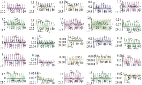
Figure-4. Exogenous Oscillations in Country 1’s Propensity to Save

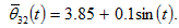
4.4. Exogenous Oscillations in Region (3, 2)’S Amenity Parameter

We now deal with how the global and national economies react to the following periodic perturbations in region (3, 2)’s amenity parameter

The simulation result is plotted in Figure 5. The global and national economies experience business cycles due to exogenous periodic changes. The global income oscillates much less than the global wealth. The two regions in country 3 experience greater changes than the other two countries. Except the lot sizes, the microeconomic variables in the economic system are affected slightly.

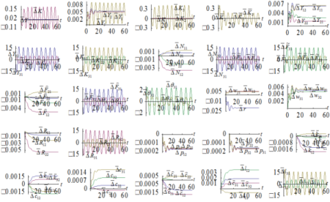
Figure-5. Exogenous Oscillations in a Region’s Amenity Parameter

4.5. Perturbations in Country 3’s Propensity to Consume Housing

We now study how the global and national economies react to the following periodic perturbations in country 3’s propensity to consume housing

The simulation result is plotted in Figure 6. The global and national economies experience business cycles. The global income oscillates less than the global wealth.

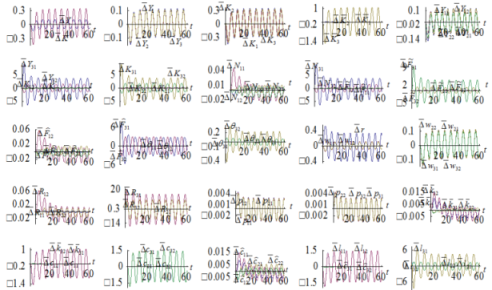
Figure-6. Perturbations in Country 3’s Propensity to Consume Housing

5. CONCLUSIONS

This paper generalized the global economic growth model with any number of countries and each country with any number of regions recently proposed by Zhang (2016). Zhang’s model extends Uzawa’s two-sector growth model to a global economy for examining dynamic interactions between international trade, national and global growth, interregional migration, wealth accumulation, and regional amenities. This study generalized Zhang’s model by allowing all the time-independent parameters to be time dependent. The generalization makes it possible to examine effects of any types of exogenous time-dependent shocks on the dynamic system cross regions over time. We simulated the model of the global economy with three countries and each country with two regions. We demonstrated the existence of equilibrium point and confirmed (local) stability of the equilibrium point. We also conducted comparative dynamic analysis with regard to exogenous periodic shocks in the total factor productivity of regions’ capital good sectors, the total factor productivities of the service sectors, the propensities to save, the amenity parameters, and the propensities to consume housing. Our comparative analysis shows how business cycles are generated by periodic exogenous shocks. The study may be extended in different ways. For instance, we may further analyze behavior of the model with other forms of production or utility functions. Moreover, households in each country should be heterogeneous. Also issues related to tax competition between countries or regions have caused great attention in economic geography. The current model is deterministic. Random factors are important in making the morel more relevant for explaining reality.

Appendix: Proving the lemma

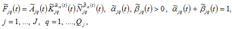
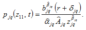
We now prove the procedure to determine the dynamics of the economic system. First, equations (2) and (4) imply

(A1)

where

Insert in from (2)

(A2)

Especially we have

(A3)

The rate of interest is determined as a unique function of and From (A2) we have

(A4)

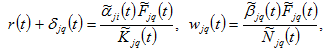
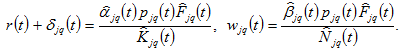
Hence we can treat all as a unique function of and Equations (A1) and (A2) imply

(A5)

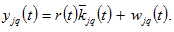
From and (1), we get

(A6)

From (16) and we get

(A7)

Inserting (4) in (A6) we have

(A8)

By (3) we have

(A9)

Substituting and (7) into (6) yields

(A10)

Applying to (A10) implies

(A11)

where

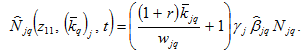
where Inserting (A11) in (18) we have

(A12)

With (A11) and (A12) we determine the population distribution within country as functions of and By and we get

(A13)

Inserting (A8) in (A9) we have

(A14)

Equations and (A11) imply

(A15)

Equations (13)-(15) imply

<

(A16)

Inserting (A1) in (A16) we get

(A17)

Substitute (A15) into (A17)

(A18)

Inserting (A14) in (A18) we have

(A19)

where

Inserting (A10) in (A19) we have

(A20)

Substituting and into equations (9) yields

(A21)

Taking derivatives of equation (A20) with respect to yields

(A22)

Inserting (A18) in (A19) we have

(A23)

With the procedure in the lemma we follow the motion of the global economic system.

Funding: The author is grateful for the financial support from the Grants-in-Aid for Scientific Research (C), Project No. 25380246, Japan Society for the Promotion of Science.

Competing Interests: The author declares that there are no conflicts of interests regarding the publication of this paper.

Contributors/Acknowledgement: The author is grateful to the constructive comments of the anonymous referee.

REFERENCES

Bond, E.W., K. Trask and P. Wang, 2003. Factor accumulation and trade: Dynamic comparative advantage with endogenous physical and human capital. International Economic Review, 44(3): 1041-1060. View at Google Scholar | View at Publisher

Brecher, R.A., Z.Q. Chen and E.U. Choudhri, 2002. Absolute and comparative advantage, reconsidered: The pattern of international trade with optimal saving. Review of International Economics, 10(4): 645-656. View at Google Scholar | View at Publisher

Deardorff, A.V. and J.A. Hanson, 1978. Accumulation and a long-run Heckscher-Ohlin theorem. Economic Inquiry, 16(2): 288-292. View at Publisher

Forslid, R. and G.I.P. Ottaviano, 2003. Trade and location: Two analytically solvable models. Journal of Economic Geography, 3(3): 229–340. View at Google Scholar 

Fujita, M., P. Krugman and A. Venables, 1999. The spatial economy. Cambridge, MA: MIT Press.

Nishimura, K. and K. Shimomura, 2002. Trade and indeterminacy in a dynamic general equilibrium model. Journal of Economic Theory, 105(1): 244-260. View at Google Scholar | View at Publisher

Oniki, H. and H. Uzawa, 1965. Patterns of trade and investment in a dynamic model of international trade. Review of Economic Studies, 32(1): 15-38. View at Google Scholar | View at Publisher

Ono, Y. and A. Shibata, 2005. Fiscal spending, relative-price dynamics, and welfare in a world economy. Review of International Economics, 13(2): 216-236. View at Google Scholar | View at Publisher

Sorger, G., 2002. On the multi-region version of the solow-swan model. Japanese Economic Review, 54(2): 146-164. View at Google Scholar | View at Publisher

Tabuchi, T., 2014. Historical trends of agglomeration to the capital region and new economic geography. Regional Science and Urban Economics, 44(C): 50–59. View at Google Scholar | View at Publisher

Uzawa, H., 1961. On a two-sector model of economic growth. Review of Economic Studies, 29(1): 47-70. View at Google Scholar | View at Publisher

Zhang, W.B., 2016. Economic globalization and interregional agglomeration in a multi-county and multi-regional neoclassical growth model. Journal of Regional Research, 34(2016): 95-121. View at Google Scholar 

Views and opinions expressed in this article are the views and opinions of the author(s), Asian Economic and Financial Review shall not be responsible or answerable for any loss, damage or liability etc. caused in relation to/arising out of the use of the content.