ECONOMIC DEVELOPMENT AND ENVIRONMENTAL CHANGE WITH ENDOGENOUS BIRTH AND MORTALITY RATES

Wei-Bin Zhang¹

¹Ritsumeikan Asia Pacific University, Japan

Keywords:Propensity to have children, Mortality rate, Birth rate, Environment, Wealth accumulation.

JEL Classification:E13, J11.

Received: 9August 2014/ Revised: 9 November 2016/ Accepted: 18November 2016/ Published: 29November 2016

Contribution/ Originality

This study makes a unique approach to dynamic relationship between economic growth and population growth with time distribution, number of children and saving as endogenous variables. The general equilibrium dynamic approach makes it possible to examine the effects of changes in the preference and technology on micro- and macro-economic variables.

1. INTRODUCTION

There are close interactions among different economic variables and government policies in modern economies. It is well-known that each of contemporary economic theories deals with some of these interactions, by neglecting many of these interactions or assuming other variables fixed. For instance, a few formal economic models study interactions between population, wealth accumulation and environment in a compact analytical framework. Nevertheless, it is evident that environmental change may affect population growth by affecting, for instance, mortality rate or life expectance. Economic growth pollutes environment and enables society to have more children. More people may either increase or reduce population. It is imperative to analyze these interactions in an integrated analytical framework, rather than studying each of the three variables by isolating possible interactional effects of the other variables. The purpose of this study is to build a general economic growth model with endogenous population, wealth and environment in a perfectively competitive economy. We show how the three variables interact over time with changes in behavior of households, firms and the government.

The study is to integrate some approaches in the literature of neoclassical economic growth theory, theory of population and theory of environmental change with the approach of household by Zhang (1993). A unique contribution of this paper is to model wealth, population and environment in a compact framework with microeconomic foundation. Wealth accumulation is built on the Solow growth model. The neoclassical growth theory based on the Solow growth model. It is well-known that the Solow one-sector neoclassical growth model is the core model for the development of neoclassical growth (e.g., (Solow, 1956; Burmeister and Dobell, 1970; Azariadis, 1993; Barro, 1995; Zhang, 2005)). There are some extensions of the Solow model by including endogenous population or/and environment as reviewed late on, this study deviates from the previous studies by modelling birth rate choice and mortality rate and by the ways of how the variables interact with each other.

We model endogenous birth and mortality rates under the influence of some important models in the literature of economic growth with population. There are many studies on birth rate and mortality rate in the literature of economic growth and population dynamics. For instance, Galor and Weil (1996) examine how fertility is dependent on factors, such as changes in gender gap in wages. Quality-quantity trade-off on children are examined by, for instance, Galor and Weil (1999) and Doepke (2004). Adsera (2005) considers the influence of labor market frictions. Hock and Weil (2012) take account of age structure. There are other formal models on determinants of fertility (Barro and Becker, 1989; Becker et al., 1990; Bosi and Seegmuller, 2012; Chu et al., 2013). There are also many studies on economic growth and mortality rate (e.g., (Robinson and Srinivasan, 1997; Chakraborty, 2004; Hazan and Zoabi, 2006; Bhattacharya and Qiao, 2007; Lancia and Prarolo, 2012) Life expectancy is influenced by factors such as health care, human capital level and environment (e.g., (Schultz, 1993;1998; Boucekkine et al., 2002; Cervellati and Sunde, 2005; Balestra and Dottori, 2012; Varvarigos and Zakaria, 2013)). There are studies on mortality rate which take account of pension systems (e.g., (Cigno and Rosati, 1996; Wigger, 1999)). There are also formal models on longevity, human capital and growth (e.g., (Kalemli-Ozcan et al., 2000; Echevarria and Iza, 2006; Heijdra and Romp, 2008; Ludwig and Vogel, 2009; Lee and Mason, 2010; Ludwig et al., 2012)). This study assumes that birth is chosen by household’s rational decision and mortality rate is related to disposable income, environment, population and environmental quality.

Endogenous population was introduced the traditional neoclassical growth theory long time ago (e.g., (Plouder, 1972; Forster, 1973)). There are many formal models on interactions between environmental change and economic growth (for instance, (Pearson, 1994; Grossman, 1995; Copeland and Taylor, 2004; Stern, 2004; Brock and Taylor, 2006; Dasgupta et al., 2006; Kijima et al., 2010)). The literature of empirical studies on relations between growth and environmental quality demonstrates different relations such as inverted U-shaped relationship, a U-shaped relationship, a monotonically increasing or monotonically decreasing relationship (Dinda, 2004; Managi, 2007; Tsurumi and Managi, 2010). No single economic theory can explain the empirical phenomena. The complexity of relations between economic development and environmental quality implies the necessity that more comprehensive economic theories are needed. The purpose of this study is to introduce endogenous environment into growth theory with endogenous population and wealth accumulation.

Time allocation between different activities is an important feature in our approach. Time is endogenous in the sense that time distribution has close interactions with other economic variables. Becker (1965) initiated formally modelling time distribution in theoretical economics. There is an immense body of empirical and theoretical literature on determinants of time distribution and relations between time distribution and economic development (e.g., (Greenwood and Hercowitz, 1991; Benhabib and Perli, 1994; Rupert et al., 1995; Ladrón-de-Guevara et al., 1997; Turnovsky, 1999; Campbell and Ludvigson, 2001)). Nevertheless, there are a few theoretical economic growth models with endogenous environment and population whichexplicitly treat work time, leisure time, and children fostering as endogenous variables. This paper introduces endogenous time into the neoclassical growth theory with environment. This paper integrates two recent papers by Zhang (2012;2014). The former study examines environment change and economic growth with time distribution between work and leisure time in the neoclassical growth theory, while the latter studies dynamic interactions between population and economic growth. This paper integrates the two models to examine dynamic interactions between wealth, environment and population with endogenous time distribution between leisure, work and children fostering. As mentioned late, our model is a synthesis of some well-known growth models. The remainder of the paper is organized as follows. Section 2 defines the economic model with endogenous capital accumulation, environmental change and population growth. Section 3 shows that the motion of the economic system is described by three differential equations and simulates the model. Section 4 carries out comparative dynamics analysis. Section 5 concludes the study.

2. THE BASIC MODEL

Following Zhang (2014) we consider that the economy consists of one production sector and one environmental sector. Exchanges take place in perfectly competitive markets. Except the assumption that environmental quality affects productivity, the production sector is similar to the standard one-sector growth model(Zhang, 2005). We consider a single good and one kind of pollutants. There are different kinds of pollutants (e.g.,(Repetto, 1987; Leighter, 1999; Nordhaus, 2000; Moslener and Requate, 2007)). We neglect heterogeneity in goods and environment for simplifying analysis. Capital of the economy is owned by the households who distribute their incomes to consume the commodity, to foster children, and to save. The labor force isfully employed bythe two sectors. The commodity is selected to serve as numeraire (whose price is normalized to 1), with all the other prices being measured relative to its price. Saving is undertaken only by households. All earnings of firms are distributed in the form of payments to factors of production.We assume a homogenous populationat time Let and represent for, respectively, the work time and leisure time of a representative household. The total work time is The total qualified labor force is

(1)

where the parameter is human capital. In this study we treat human capital fixed.

2.1. The Production Sector

Following Zhang (2012) we assume that environmental quality affects economic productivities (see also, (Gradus and Smulders, 1996; Grimaud, 1999; Ono, 2002). We specify production function of the production sector as follows

(2)

where is the output level of theproduction sector at time is a function of the environmental quality measured by the level of pollution, is total productivity, and andare respectively output elasticities of capital and labor. Let and represent respectively the rateof interestand wage rate. We use to stand for the fixed tax rate,The marginal conditions for firms to maximize their profits are as follows

(3)

where is the fixed depreciation rate of physical capital and

2.2. Consumer Behaviors

Consumers decide time distribution, consumption level of commodity, number of children, and amount of saving. Different from the traditional approaches to household behavior, we use an alternative approach to household proposed by Zhang (1993). Per capita wealth is denoted by We have where is the total capital stock. The per capita disposable current income which is the sum of the interest payment and the wage payment after taxation is given by

where and are respectively the tax rates on the interest payment and wage income. We call the current income in the sense that it comes from consumers’ payment for efforts and consumers’ current earnings from ownership of wealth. In Zhang’s approach the disposable income is the sum of the current income plus the value of the wealth help by the household. That is

We use and to represent the birth rate and the cost of birth. There are many factors which may influence costs of bringing up children. Following Zhang (2014) we assume that children will have the same level of wealth as that of the parent. Following this assumption, we have the following relation between cost and birth rate

(4)

It should the noted that the fertility choice model of Barro and Becker (1989) takes account of the cost of consumption goods by children.We assume that the time spent on children fostering is proportional to the birth rate. The relation between birth rate and parent’s time on raising children is specified as follows

(5)

The specified function form implies that if the parents want more children, they spend more time on child caring. Here, we neglect possible increasing return to scale in children caring. It should be noted that Tournemaine and Luangaram (2012) use the following technology of production of children: where and are parameters. If then our approach is the same as the equation accepted by Tournemaine and Luangaram.

The household distributes the total available budget between saving,consumption of goods, and bearing children, The budget constraint is

(6)

where is the tax rate on the consumption. We omit possible effects of consumers’ awareness on environmental change. For instance, it is possible that consumers may affect environment and thus productivities by choosing more environment-friendly goods.

The total available time is distributed between work, child fostering, and leisure pursuit. The family is faced with the following time constraint

(7)

where is the total available time for leisure, work and children caring. Substituting (7) into (6) yields

(8)

where and

The right-hand side is the “potential” income that the family can obtain by spending all the available time on work. The left-hand side is the sum of the consumption cost, the saving, the opportunity cost of bearing children, and opportunity cost of leisure. Insert (5) in (8)

(9)

whereThe variable is the opportunity cost of children fostering.

We now model how the household makes decision on the number of children. Following Barro and Becker (1989) who assume that the parents’ utility is dependent on the number of children, we include birth rate into utility function (see also, Chu et al. (2013);Razin and Ben-Zion (1975);Yip and Zhang (1997)). Rather than the traditional Ramsey approach, we use the utility function proposed by Zhang (1993). We assume that the utility is dependent on and as follows

where is called the propensity to consume, the propensity to own wealth, the propensity to use leisure time, the propensity to have children, and is the elasticity of environmental quality. The specified utility implies that utility is negatively related to pollution (see also (Balcao, 2001; Nakada, 2004)). According to Munro (2009) “environmental economics has been slow to incorporate the full nature of the household into its analytical structures. … [A]n accurate understanding household behavior is vital for environmental economics.” The first-order condition of maximizing subject to(9) yields

(10)

where

2.3. The Birth and Mortality Rates and Population Dynamics

According to the definitions, the population change is given by

(11)

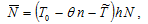
where is the mortality rate. They consider mortality rate constant. In the Haavelmo model, the mortality rate is negatively related to per capita income(Haavelmo, 1954; Stutzer, 1980). In this study we assume that the mortality rate is related to the disposable income, population and to level of pollutants in the following way

(12)

whereand are parameters. We call the mortality rate parameter. As in the Haavelmo model, an improvement in living conditions implies that people live longer. This implies a negative relation between the disposable income and mortality rate, that is, The term takes account of possible influences of environmental quality on mortality. It is reasonable to assume that as environment is deteriorated, mortality rate tends to rise We don’t specify the sign of as the population may be positively or negatively related to mortality rate. Insert (10) and (12) in (11)

(13)

The equation describes the population dynamics. For simplicity of analysis, this study does not describe the population change, we should also model the age structure. Like in most of the models in continuous time in the literature of economic growth and population change, for simplicity of analysis we don’t deal with complicated issues related to the age structure in this stage of research.

2.4. Dynamics of Wealth Accumulation

According to the definition of the change in the household’s wealth is given by

(14)

The equation simply states that the change in wealth is equal to saving minus dissaving.

2.5. Environmental Change

The environmental change is based on Zhang (2012). We assume that dynamics of the stock of pollutants are affected by production and consumption. We specify the dynamics of the stock of pollutants as follows

(15)

where, and are positive parameters and

(16)

whereand are positive parameters, and is a function of We assume that emission of pollutants during production processes is linearly positively proportional to the output level. The households creases units of waste in consuming one unit of the good (John and Pecchenino, 1994; John et al., 1995; Prieur, 2009). The term is the rate that the nature purifies environment, where is called the rate of natural purification. We use the term, in to reflect that that the purification rate of environment is positively related to capital and labor inputs. The function means that the purification efficiency is related to the stock of pollutants.

2.6. The Behavior of the Environmental Sector

In this study we consider that the environmental sector is financially supported by the government. The sector decides the number of labor force and the level of capital employed. The government’s tax revenue consists of the tax incomes on the production sector, consumption, wage income and wealth income. Hence, the government’s income is given by

(17)

We assume that all the tax incomes are spent on environment. For simplicity, we assume that all the revenue of the government is spent on protecting environment. The environmental sector’s budget is

(18)

According to Zhang (2014)the environmental sector employs labor and uses capital in such a way that the purification rate achieves its maximum under the given budget constraint. The sector’s optimal problem is given by

s.t.: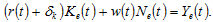

The optimal solution is

(19)

where

2.7. Full Employment of Production Factors

We use and to respectivelystand for the labor force and capital stocks employed by the environmental sector. As full employment of labor and capital is assumed, we have

(20)

2.8. Demand For and Supply of Goods

The national saving is the sum of the households’ saving. As output of the capital goods sector is equal to the net savings and the depreciation of capital stock, we have

(21)

where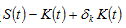 is the sum of the net saving and depreciation, 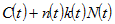is the total expenditure and

We have thus built the dynamic model. It should be noted that the model is general in the sense that the Solow model and the Haavelmo model can be considered as special cases of our model. Moreover, as our model is based on the some well-known mathematical models and includes some features which no other single theoretical model explains, we should be able to explain some interactions which other formal models fail to explain. We now examine dynamics of the model.

3. THE DYNAMICS AND ITS PROPERTIES

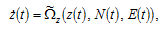
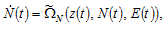
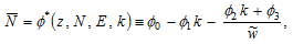
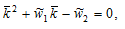
We built the growth model with endogenous wealth, population and environment. The model contains many variables and these variables are interrelated to each other in complicated ways. It is difficult to get analytical properties of the nonlinear differential equations. For illustration, we simulate the model to demonstrate how variables change over time. First, we introduce, 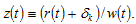We show that the dynamics can be expressed by a three-dimensional differential equations system with and as the variables.

Lemma

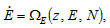
The dynamics of the economic system is governed by the three dimensional differential equations

(22)

where the functions and are functions of and defined in the Appendix. Moreover, all the other variables are determined as functions of and at any point in time by the following procedure: by (A16)→ and by (A8) → and by (A2) → and by (A1) → by definition → and by (10) → → by (12) → by (7) → by (1) → by (2) → by (19) → by (16).

We have three nonlinear differential equations with three variables, and As the expressions are too complicated, it is difficult to obtain analytical solutions or general properties of the nonlinear dynamic system. For illustration we simulate the model to plot motion of the economic system. In the remainder of this study, we specify the depreciation rates by The available time is The depreciation rate of physical capital is often fixed around in economic studies. Environmental effects on the productivities are as follows

We specify the other parameters as follows

(23)

The propensity to save is and the propensity to consume goods is The propensity to have children is and the propensity to have leisure time is lower than the propensity to have children. The technological parameters of the two sectors are specified at and The human capital level is The tax rates are all fixed at 5 percent. We specify initial conditions as follows

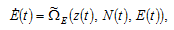
The simulation result is plotted in Figure 1. The figure shows that both the birth rate and mortality rate are increased from their initial values. Nevertheless, the mortality rate rises faster than the birth rate. The population is consequently reduced. The total capital stock and total labor input fall over time. The output levels, labor and capital inputs of the two sectors are reduced. The wealth per household is reduced. As the household has less wealth and the wage rate falls, the opportunity cost of children fostering falls, although the household works more hours. The household spends more hours on work and children fostering, and spends less time on leisure. The environmental quality is deteriorated initially and then falls.

Figure-1. The Motion of the Economic System

The simulation demonstrates that the dynamic system approaches an equilibrium point. We list the equilibrium values of the variables as follows

(24)

We calculate the three eigenvalues at this equilibrium point as follows

As the three eigenvalues are real and negative, the unique equilibrium point is stable. Hence, the system always approaches its equilibrium if it is not far from the equilibrium point. We can conduct comparative dynamic analysis near this equilibrium point.

4. COMPARATIVE DYNAMIC ANALYSIS IN SOME PARAMETERS BY SIMULATION

We have demonstrated how to follow the motion of the national economy over time from any state. It is imperative to examine effects of parameter changes on paths of economic growth. To present impact of changes in some parameters on dynamic processes of the system, we use a variable to stand for the change rate of the variable, in percentage due to changes in the parameter value.

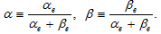
4.1. The Propensity to have Children Enhanced

Modern economies offer great varieties of goods and services and makes different life styles possible. One of changes in modern societies is the propensity to have children. One may find many determinants of the propensity to have children. Although we are not concerned why the propensity is shifted, we examine what will happen to the economic system if the propensity to have children is enhanced as follows: The simulation results are plotted in Figure 2. When people increase their propensity to have children, the birth rate is enhanced. The population and work time are increased. Consequently the total labor supply is increased. The household has less leisure time and spends more time on children fostering. The environment is deteriorated in association with rising population. The total capital is increased, even though wealth per household is lessened. The net impact of rising population and falling in wealth per household on the national capital is positive. The wage rate and opportunity cost of children fostering are lowered. The output levels, labor inputs, and capital inputs of the two sectors are all increased. The rate of interest is increased. The consumption level of goods is reduced. It should be noted that the model by Varvarigos and Zakaria (2013) predicts a fertility decline along the process of economic growth. The two-period overlapping-generations model by Strulik (2008) predicts an inverted U-shape relationship between fertility and income. Acemoglu and Johnson (2007)try to analyze the impact of life expectancy on economic growth. There is no evidence of a positive effect. It is also observed that there is a decline of the fertility rate alone the process of economic development (e.g., (Kirk, 1996; Ehrlich and Lui, 1997; Galor, 2012)). Although this study accepts an analytical framework different from the traditional models, our analyses show that change directions of the birth rate and mortality rate are determined by different forces.

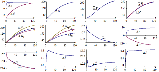
Figure-2. The Propensity to Have Children Being Enhanced

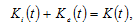
4.2. A Rise in Human Capital

Relations between environmental and population growth have caused much attention in public as well as academic discussions. Although this study does not take account of endogenous human capital and education cost, we are interested in what will happen if human capital is improved as follows: The simulation results are plotted in Figure 3. The time distribution is slightly affected by the change in human capital. The wage income is increased, though the wage rate per qualified unit time falls as the total capital stock is increased. The consumption levels of goods and wealth per household are enhanced in association in rise in the wage income. It is more expensive to have children in terms of opportunity cost of children fostering. Although the birth rate is slightly affected, the mortality rate is decreased. The net impact of almost invariant birth rate and reduced mortality rate increases the population. The total labor force is augmented as the population is increased, human capital is improved, and the work time is almost not affected. The net impact of rising population (which tends to enhance rate of interest) and rising total capital stock (which tends to lower rate of interest) increases rate of interest. The output levels, labor inputs, and capital inputs of the two sectors are all increased. The environmental quality is deteriorated as the economic conditions are improved and the population is increased.

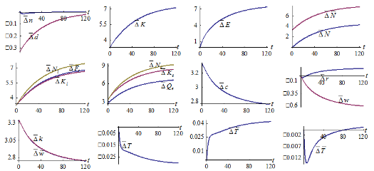
Figure-3. A Rise in Level of Human Capital

4.3. Consumption Tax Being Enhanced

We now examine effects of changes in different taxes on economic growth and population change. It should be noted that all the tax income is spent on environmental improvement in this study and is not directly used for influencing population change. We consider the following change in the tax rate on consumption: The simulation results are plotted in Figure 4. The level of consumption is reduced. As more resource is spent on environmental improvement, the environmental quality is improved. More labor and capital inputs are employed by the environmental sector. The output of the environmental sector is increased. The work time is reduced and the leisure time is reduced. The time for children fostering is slightly affected. The birth rate is slightly increased and the mortality rate is decreased. The net impact on birth and mortality rates increases the population. The total labor force is augmented. The wage income and the wage rate per qualified unit time are increased. The wealth per household is enhanced in association in fall in the level of consumption. It is more expensive to have children in terms of opportunity cost of children fostering as wealth per household and wage rate are increased. The national capital stock is augmented. The rate of interest is enhanced. The output level, labor input, and capital input of the production sector fall initially and rise in the long term.

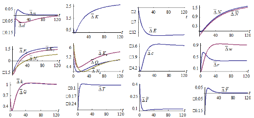
Figure-4. Consumption Tax Being Enhanced

4.4. Tax Rate on Income from Interest of Wealth Being Enhanced

We examined the effects of a rise in consumption tax rate on economic growth and population change. We now study what will happen if consider the following change in the tax rate on consumption: The simulation results are plotted in Figure 5. The levels of wealth and consumption are increased initially but soon reduced. The time on children fostering and leisure time are reduced and the work time is increased. As more resource is spent on environmental improvement, the environmental quality is improved. More labor and capital inputs are employed by the environmental sector. The output of the environmental sector is increased. The birth rate is reduced and the mortality rate is slightly increased. The net impact on birth and mortality rates lessens the population. The total labor force is decreased. The wage rate per qualified unit time is lowered initially and augmented slightly in the long term. The opportunity cost of children fostering is reduced. The national capital stock is slightly increased and is soon reduced. The rate of interest is enhanced. The output level, labor input, and capital input of the production sector fall. By comparing Figures 4 and 5 we conclude that changes in the tax rates on consumption and interest income have different effects on population growth and economic development.

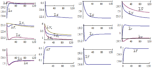
Figure-5. Tax Rate on Income from Interest of Wealth Being Enhanced

4.5. Tax Rate on the Production Sector’s Output Being Augmented

We consider the following change in the tax rate on the production sector’s output: 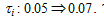The simulation results are plotted in Figure 6. The output level, labor input, and capital input of the production sector fall. As more resource is spent on environmental improvement, the environmental quality is improved. More labor and capital inputs are employed by the environmental sector. The output of the environmental sector is increased. The level of consumption is reduced. The work time is reduced and the leisure time is reduced. The time for children fostering is reduced initially and is slightly affected in the long term. The birth rate is reduced and the mortality rate is increased slightly. The net impact on birth and mortality rates reduces the population. The total labor force is lowered. The wage income and the wage rate per qualified unit time are reduced. The wealth per household is. It is less expensive to have children in terms of opportunity cost of children fostering. The national capital stock is reduced. The rate of interest is reduced initially and increased in the long term. We simulated effects of the following rise in the wage rate: 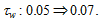We do not list the results as the effects are similar to these due to the change in

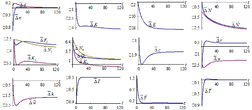
Figure-6. Tax Rate on the Production Sector’s Output Being Augmented

4.6. Environment Having Stronger Impact on Productivity of the Production Sector

We examine what will happen when environment has stronger impact on productivity of the production sector as follows: The simulation results are plotted in Figure 7. As the productivity falls, the output level, labor input, and capital input of the production sector fall. As more resource is spent on environmental improvement, the economy experiences environmental improvement. The environmental sector employs more labor and capital inputs. The output of the environmental sector is consequently augmented increased. The work time is reduced and the leisure time is reduced. The time for children fostering is slightly affected. The level of consumption is reduced. The birth rate is reduced and the mortality rate is increased slightly. The net impact on birth and mortality rates reduces the population. The total labor force is lowered. The wage income and the wage rate per qualified unit time are reduced. The wealth per household is. It is less expensive to have children in terms of opportunity cost of children fostering. The national capital stock is reduced. The rate of interest is reduced initially and increased in the long term. It should be noted that the effects are similar to the effects caused by the rise in the tax rate on the production sector.

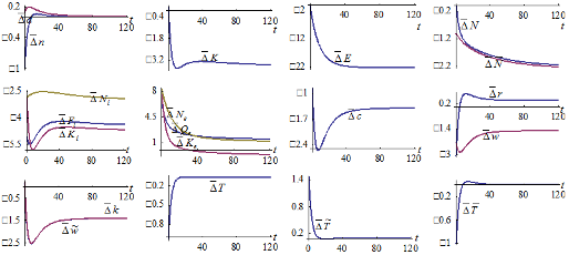
Figure-7. Environment Having Stronger Impact on Productivity of the Production Sector

4.7. A Stronger Impact of Environment on the Mortality Rate

We consider that environmental change affects mortality. We are now concerned with what will happen if environment has stronger impact on mortality rate as follows: The simulation results are plotted in Figure 8. The mortality rate is increased. The birth rate is almost not affected. The population is reduced. The time distribution is slightly affected. The total labor supply is increased. The wage income and the wage rate per qualified unit time are increased. The consumption levels of goods and wealth per household are enhanced in association in rise in the wage income. It is more expensive to have children in terms of opportunity cost of children fostering. The total labor force is augmented. The net impact of rising population and rising total capital stock lowers rate of interest. The output levels, labor inputs, and capital inputs of the two sectors are all increased. The environmental quality is improved as the population is reduced.

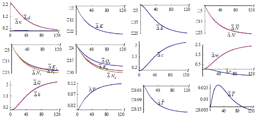
Figure-8. A Stronger Impact of Environment on the Mortality Rate

5. CONCLUDING REMARKS

This study examined dynamic interactions among population growth, wealth accumulation, and environmental dynamics with endogenous time distribution among work, leisure and children fostering. We built a model on the basis of some well-known models within a compact framework. The wealth accumulation and economic production were built on the Solow growth model. We introduced the dynamics of birth and mortality rates under the influence of the Haavelmo population model and the Barro-Becker fertility choice model. The environmental dynamics was modelled on the basis of some well-known neoclassical growth models with environmental change. We modelled the time distribution between work time, leisure time and time of children fostering with an alternative approach to household by Zhang. The study succeeded in synthesizing different economic forces in a compact framework mainly because we applied the approach by Zhang. We showed that the motion of the economic system is described by three nonlinear differential equations. As dynamic analysis of the nonlinear system is too complicated, we simulated the model. We plotted the motion of the system and demonstrated the existence of an equilibrium point. We studied the effects of changes on the motion of the economic system in the propensity to have children, the tax rates, and the strength of impact by environment on mortality rate. The simulation demonstrates some dynamic interactions among the variables which can be predicted neither by the neoclassical growth theory nor by the traditional economic models of environmental change because our model provides an analytical framework for analyzing interactions among multiple variables. As the model is based on the basic ideas in some economic theories and each of these theories has a huge amount of literature, it is straightforward to extend the model on the basis of the literature. For instance, we may introduce multiple capital and education into the model. It is imperative to study family structure and economic structure for understanding relations among growth, environmental change and population growth (see, for instance, (Dinda, 2004; Hamilton and Zilberman, 2006)).

Appendix:Proving Lemma 1

We now confirm the three-dimensional differential equations in lemma. From (3) and (19), we obtain

(A1)

whereFrom (2) and (3) we have

(A2)

where we also use (A1). We thus determine and as functions of and Insert (A1) in (20)

(A3)

From (1) and (12), we have

(A4)

where we use Insert (10) in (A4)

(A5)

Insert 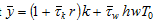in (A5)

(A6)

where

Insert (A6) and in (A9)

(A7)

Solve (A7)

(A8)

From (20) we have

(A9)

where Insert (10) and (15) in (A16)

(A10)

Insert in (A10)

(A11)

whereSubstituting (A1) into (A18) yields

(A12)

where

Insert (A8) in (A12)

(A13)

where

Insert (A6) and in (A13)

(A14)

where

Insert and in (A14)

(A15)

where

Solve (A15) with regard to

(A16)

In our simulation we have a unique meaningful solution as follows

We determine all the variables as functions of and as in the lemma.

From this procedure, (5) and (18), it is straightforward to show that the motion of environment and the population can be expressed as function of and at any point in time

(A17)

We now show that change in can also be expressed as a differential equation in terms of and From (14), we have

(A18)

Taking derivatives of (A16) for one of the two solutions with respect to time, we have

(A19)

Where we also use (A17). From (A18) and (A19), we solve

(A20)

The three differential equations (A17) and (A20) contain three variables and We thus proved the lemma.

Funding: The author is grateful for the financial support from the Grants-in-Aid for Scientific Research (C), Project No. 25380246, Japan Society for the Promotion of Science.

Competing Interests: The author declares that there are no conflicts of interests regarding the publication of this paper.

Contributors/Acknowledgement: The author is grateful to the constructive comments of the two anonymous referees.

REFERENCES

Acemoglu, D. and S. Johnson, 2007. Disease and development: The effect of life expectancy on economic growth. Journal of Political Economy, 115(6): 925-985.

Adsera, A., 2005. Vanishing children: From high unemployment to low fertility in developed countries. American Economic Review, 95(2): 189-193.

Azariadis, C., 1993. Intertemporal macroeconomics. Oxford: Blackwell.

Balcao, A., 2001. Endogenous growth and the possibility of eliminating pollution. Journal of Environmental Economics and Management, 42(3): 360-373.

Balestra, C. and D. Dottori, 2012. Aging society, health and the environment. Journal of Population Economics, 25(3): 1045-1076.

Barro, R.J. and G.S. Becker, 1989. Fertility choice in a model of economic growth. Econometrica, 57(2): 481-501.

Barro, R.J.S.-i.-M., X., 1995. Economic growth. New York: McGraw-Hill, Inc.

Becker, G., K.M. Murphy and R. Tamura, 1990. Human capital, fertility, and economic growth. Journal of Political Economy, 98(5): S12-S37.

Becker, G.S., 1965. A theory of the allocation of time. Economic Journal, 75(299): 493-517.

Benhabib, J. and R. Perli, 1994. Uniqueness and indeterminacy: On the dynamics of endogenous growth. Journal of Economic Theory, 63(1): 113-142.

Bhattacharya, J. and X. Qiao, 2007. Public and private expenditures on health in a growth model. Journal of Economic Dynamics and Control, 31(8): 2519–2535.

Bosi, S. and T. Seegmuller, 2012. Mortality differential and growth: What do we learn from the barro-becker model? Mathematical Population Studies, 19(1): 27-50.

Boucekkine, R., D. De la Croix and O. Licandro, 2002. Vintage human capital. Demographic trends, and endogenous growth. Journal of Economic Growth, 104(2): 340-375.

Brock, W. and M.S. Taylor, 2006. Economic growth and the environment: A review of theory and empirics. In Durlauf, S. and Aghion, P. (Eds.), The handbook of economic growth. Amsterdam: Elsevier.

Burmeister, E. and A.R. Dobell, 1970. Mathematical theories of economic growth. London: Collier Macmillan Publishers.

Campbell, J.Y. and S. Ludvigson, 2001. Elasticities of substitution in real business cycle model with home production. Journal of Money, Credit, and Banking, 33(4): 847-875.

Cervellati, M. and U. Sunde, 2005. Human capital formation, life expectancy, and the process of development. American Economic Review, 95(5): 1653-1672.

Chakraborty, S., 2004. Endogenous lifetime and economic growth. Journal of Economic Theory, 116(1): 119-137.

Chu, A.C., G. Cozzi and C.H. Liao, 2013. Endogenous fertility and human capital in a schumpeterian growth model. Journal of Population Economics, 26(1): 181-202.

Cigno, A. and F.C. Rosati, 1996. Jointly determined saving and fertility behaviour: Theory and estimates for Germany, Italy, UK and USA. European Economic Review, 40(8): 1561-1589.

Copeland, B. and S. Taylor, 2004. Trade, growth and the environment. Journal of Economic Literature, 42(1): 7-71.

Dasgupta, S., K. Hamilton, K.D. Pandey and D. Wheeler, 2006. Environment during growth: Accounting for governance and vulnerability. World Development, 34(9): 1597-1611.

Dinda, S., 2004. Environmental Kuznets curve hypothesis: A survey. Ecological Economics, 49(4): 431-455.

Doepke, M., 2004. Accounting for fertility decline during the transition to growth. Journal of Economic Growth, 9(3): 347-383.

Echevarria, C.A. and A. Iza, 2006. Life expectancy, human capital, social security and growth. Journal of Public Economics, 90(12): 2324-2349.

Ehrlich, I. and F. Lui, 1997. The problem of population and growth: A review of the literature from malthus to contemporary models of endogenous population and endogenous growth. Journal of Economic Dynamics and Control, 21(1): 205-242.

Forster, B.A., 1973. Optimal consumption planning in a polluted environment. Economic Record, 49(4): 534-545.

Galor, O., 2012. The demographic transition: Causes and consequences. Cliometrica, 6(6): 1-28.

Galor, O. and D. Weil, 1999. From Malthusian stagnation to modern growth. American Economic Review, 89(2): 150-154.

Galor, O. and D.N. Weil, 1996. The gender gap, fertility, and growth. American Economic Review, 86(3): 374-387.

Gradus, R. and S. Smulders, 1996. The trade-off between environmental care and long-term growth-pollution in three prototype growth models. Journal of Economics, 58(1): 25-51.

Greenwood, J. and Z. Hercowitz, 1991. The allocation of capital and time over the business cycle. Journal of Political Economy, 99(6): 1188-1214.

Grimaud, A., 1999. Pollution permits and sustainable growth in a schumpeterian model. Journal of Environmental Economics and Management, 38(3): 249-266.

Grossman, G.M., 1995. Pollution and growth: What do we know? In Goldin, I. and Winters, L.A. (Eds.), The economics of sustainable development. Cambridge: Cambridge University Press.

Haavelmo, T., 1954. A study in the theory of economic evolution. Amsterdam: North-Holland.

Hamilton, S.F. and D. Zilberman, 2006. Green markets, eco-certification, and equilibrium fraud. Journal of Environmental Economics and Management, 52(3): 627-644.

Hazan, M. and H. Zoabi, 2006. Does longevity cause growth? A theoretical critique. Journal of Economic Growth, 11(4): 363-376.

Heijdra, B.J. and W.E. Romp, 2008. A life-cycle overlapping-generations model of the small open economy. Oxford Economic Papers, 60(1): 88-121.

Hock, H. and D.N. Weil, 2012. On the dynamics of the age structure, dependency, and consumption. Journal of Population Economics, 25(3): 1019-1043.

John, A. and R. Pecchenino, 1994. An overlapping generation model of growth and the environment. Economic Journal, 104(427): 1393-1410.

John, A., R. Pecchenino, Schimmelpfenning and S. Schreft, 1995. Short-lived agents and the long-lived environment. Journal of Public Economics, 58(1): 127-141.

Kalemli-Ozcan, S., H.E. Ryder and D.N. Weil, 2000. Mortality decline, huma capital investment, and economic growth. Journal of Development Economics, 62(1): 1-3.

Kijima, M., K. Nishide and A. Ohyama, 2010. Economic models for the environmental Kuznets curve: A survey. Journal of Economic Dynamics & Control, 34(7): 1187-1201.

Kirk, D., 1996. Demographic transition theory. Population Studies, 50(1996): 361–387.

Ladrón-de-Guevara, A., S. Ortigueira and M.S. Santos, 1997. Equilibrium dynamics in two-sector models of endogenous growth. Journal of Economic Dynamics and Control, 21(1): 115-143.

Lancia, F. and G. Prarolo, 2012. A politico-economic model of aging, technology adoption and growth. Journal of Population Economics, 25(3): 989-1018.

Lee, R. and A. Mason, 2010. Fertility, human capital, and economic growth over the demographic transition. European Journal of Population, 26(2): 159-182.

Leighter, J.E., 1999. Weather-induced changes in the trade-of between SO2 and NOx at large power plants. Energy Economics, 21(6): 239-259.

Ludwig, A., T. Schelkle and E. Vogel, 2012. Demographic change, human capital and welfare. Review of Economic Dynamics, 15(1): 94-107.

Ludwig, A. and E. Vogel, 2009. Mortality, fertility, education and capital accumulation in a simple OLG economy. Journal of Population Economics, 23(2): 703-735.

Managi, S., 2007. Technological change and environmental policy: A study of depletion in the oil and gas industry. Cheltenham: Edward Elgar.

Moslener, U. and T. Requate, 2007. Optimal abatement in dynamic multi-pollutant problems when pollutants can be complements or substitutes. Journal of Economic Dynamics & Control, 31(7): 2293-2316.

Munro, A., 2009. Introduction to the special issue: Things we do and don’t understand about the household and the environment. Environmental and Resources Economics, 43(1): 1-10.

Nakada, M., 2004. Does environmental policy necessarily discourage growth? Journal of Economics, 81(3): 249-268.

Nordhaus, W.D., 2000. Warming the world, economic models of global warming. MA.,Cambridge: MIT Press.

Ono, T., 2002. Emission permits on growth and the environment. Environmental and Resources Economics, 20(1): 75-87.

Pearson, P.J., 1994. Energy, externalities and environmental quality: Will development cure the ills it creats? Energy Studies Review, 6(3): 199-216.

Plouder, G.C., 1972. A model of waste accumulation and disposal. Canadian Journal of Economics, 5(1): 119-125.

Prieur, F., 2009. The environmental Kuznets curve in a world of irreversibility. Economic Theory, 40(1): 57-90.

Razin, A. and U. Ben-Zion, 1975. An intergenerational model of population growth. American Economic Review, 65(5): 923-933.

Repetto, R., 1987. The policy implications of non-convex environmental damages: A smog control case. Journal of Environmental Economics and Management, 14(1): 13-29.

Robinson, J.A. and T.N. Srinivasan, 1997. Long-term consequence of population growth: Technological change, natural resources, and the environment. In handbook of population and family economics, edited by Rozenzweig, M.R. and Stark, O. Amsterdam: North-Holland.

Rupert, P., R. Rogerson and R. Wright, 1995. Estimating substitution elasticities in household production models. Economic Theory, 6(1): 179-193.

Schultz, P.T., 1993;1998. Mortality decline in the low-income world: Causes and consequences. American Economic Review, 83(2): 337-342.

Solow, R., 1956. A contribution to the theory of growth. Quarterly Journal of Economics, 70(1): 65-94.

Stern, D.I., 2004. The rise and fall of the environmental Kuznets curve. World Development, 32(8): 1419-1439.

Strulik, H., 2008. Geography, health, and the pace of demo-economic development. Journal of Development Economics, 86(1): 61–75.

Stutzer, M., 1980. Chaotic dynamics and bifurcation in a macro economics. Journal of Economic Dynamics and Control, 2(1980): 253-273.

Tournemaine, F. and P. Luangaram, 2012. R&D, human capital, fertility, and growth. Journal of Population Economics, 25(3): 923-953.

Tsurumi, T. and S. Managi, 2010. Decomposition of the environmental Kuznets curve: Scale, technique, and composition effects. Environmental Economics and Policy Studies, 11(1): 19-36.

Turnovsky, S.J., 1999. Fiscal policy and growth in a small open economy with elastic labor supply. Canadian Journal of Economics, 32(5): 1191-1214.

Varvarigos, D. and I.Z. Zakaria, 2013. Endogenous fertility in a growth model with public and private health expenditures. Journal of Population Economics, 26(1): 67-85.

Wigger, B.U., 1999. Pay-as-you-go financed public pensions in model of endogenous growth and fertility. Journal of Population Economics, 12(4): 625-640.

Yip, C. and J. Zhang, 1997. A simple endogenous growth model with endogenous fertility: Indeterminacy and uniqueness. Journal of Population Economics, 10(1): 97-100.

Zhang, W.B., 1993. Woman’s labor participation and economic growth - creativity, knowledge utilization and family preference. Economics Letters, 42(1): 105-110.

Zhang, W.B., 2005. Economic growth theory. London: Ashgate.

Zhang, W.B., 2012. Capital accumulation, technological progress and environmental change in a three-sector growth model. International Journal of Information Systems and Social Change, 3(3): 1-18.

Zhang, W.B., 2014. Endogenous population with human and physical capital accumulation. International Review of Economics, 61(3): 231-252.

Views and opinions expressed in this article are the views and opinions of the author(s), Asian Journal of Economic Modellingshall not be responsible or answerable for any loss, damage or liability etc. caused in relation to/arising out of the use of the content.