


ASYMMETRIC EFFECTS OF CHINA’S MONETARY POLICY ON THE STOCK MARKET: EVIDENCE FROM A NONLINEAR VAR MODE

1,2Subject Group of Economics and Finance, Portsmouth Business School, University of Portsmouth, Portsmouth PO1 3DE, Hampshire, United Kingdoms
ABSTRACT
This study uses Markov switching vector autoregression (MS-VAR) model to explore the asymmetric effects of China’s monetary policy on the stock market in the bull market and the bear market. With China’s economy in a rapid development, China’s stock market as the main representative of the virtual economy has attracted large assets. Since 1990 to the present, China’s stock market has experienced several times states’ change between the bull market and bear market. The results indicate that China’s quantity-based direct instrument and price-based indirect instrument have asymmetric effects on the stock market in the bull market and the bear market. Moreover, the relationship between China’s economy and stock market exist a degree of dichotomy. Furthermore, China’s monetary policy has stronger effects on the bull market than the bear market.
Keywords:China’s monetary policy China’s economy Stock market Bull market Bear market Quantity-based direct monetary instruments Price-based indirect monetary instruments Asymmetric effects MS-VAR model.
ARTICLE HISTORY: Received:10 April 2018. Revised:7 May 2018. Accepted:10 May 2018. Published:23 May 2018.
Contribution/ Originality:Based on the framework of monetary policy and stock market, this study uses the MS-VAR model to explore the China’s monetary policy has asymmetric effects on the stock market. And, this study identifies the effects of China’s monetary policy on the bull market are stronger than bear market.
1. INTRODUCTION
Monetary policy is one of the most important economic instruments for regulating the financial market’s development. The ultimate targets of monetary policy are price stability, full employment, economic growth, and financial market stability. The transmission mechanism and targets of monetary policy are inevitably reached through the financial market and capital market (Bernanke and Vincent, 2004). Since the 20th century, the economic globalization has stimulated the development of the scale and intensiveness of the financial market in developed economies and emerging economies. The continuous improvement of the financial market has led to the continuous expansion of financial instruments and financial skills.
Generally, monetary policy affects the stock market by three steps. The first step is that monetary policy is used by the central bank to affect financial institutions and financial markets. The central bank uses the monetary instruments to affect financial institutions’ reserves, financing costs, and credit capacity. The second step is that monetary policy is used by the commercial banks and other financial institutions to stimulate enterprises and residents. Commercial banks and other financial institutions adjust in accordance with monetary policy to affect the consumption, saving, investment and other economic activities. The third step is monetary policy via the non-financial sector, where economic actors control social-economic variables, such as total expenditure, total output, price, and employment. Through capital flow, monetary policy has positive effects on resource allocation, risk management and corporate governance (Rigobon and Sack, 2001; Castelnuovo and Nistico, 2010; Milani, 2011). The relationship between monetary policy and the stock market are closer than before. The central bank considers the effects of monetary policy on the stock market. Moreover, there are some literature that argue that monetary policy has asymmetric effects. Thorbecke (1997) uses the vector auto-regression model to analyze the federal funds rate, the stock yields, industrial added value and other variables have asymmetric effects. Bernanke and Kutter (2005) find that the unexpected cutting of federal funds rate on the stock market has a significant and positive result of rising stock prices. Hyde and Bredin (2005) apply the smooth transit regression model to test the macroeconomic variables of Canada, France, Japan, UK and USA and find that there exist a non-linear relationship between macroeconomy with stock market. Almeida and Campello (2007) and Livdan et al. (2009) claim that if the financing channel of investment is constrained, monetary policy has asymmetric effects on the financial markets. Brandley and Jansen (2004) compare the forecasting capability of linear model and nonlinear model and show that the nonlinear model has a better forecasting effect than linear model. In China, monetary policy has exercised the main targets and instruments after 1998’s monetary policy innovation. Before the economic transformation, China’s economy implemented a highly centralized and unified planned system in the long-term. Based on this condition, China’s monetary policy has been in a subordinate status. Institutional reform and economic development have promoted the effects of China’s monetary policy and deepened China’s financial market development. After 2002, China’s monetary authority has established a relatively completed monetary policy, which meant that the People’s Bank of China frequently uses quantity-based direct monetary instruments and price-based indirect monetary instruments to operate and regulate the economy. China’s stock market has enlarged in scale since establishing the Shanghai Stock Exchange and Shenzhen Stock Exchange. Due to China’s financial market development, the Chinese stock market has become the second largest market in the world. Stock market has played important role in China’s economic development as the relationship between China’s monetary policy, economic development, and the stock market have become closer than before.
According to the related economic theories and test criteria, this study establishes a four-variable MS-VAR model in two regimes to shed light on the asymmetric effects of China's monetary policy on the stock market. One is in the bull market, and the other being in the bear market. This study indicates that China's monetary policy, stock market returns and economic output have a significant non-linear relationship. Moreover, results show that China’s monetary policy has asymmetric effects on the stock market in a bull market and a bear market. This study makes three contributions to the extant literature. Firstly, this study uses the MS-VAR model to certificate the effects monetary policy on the closed state of China’s stock market are asymmetric. Second, to the best of my knowledge, this is the first study which empirically certificates there is a certain degree of the dichotomy between China's stock market with the real economy. Third, this study identifies the effects of China’s monetary policy on the bull market are stronger than the bear market. This research findings also have important research implications. First, this study can theoretically analyse the information response capacity of the stock market under different market operation stages. This study tests the specific impact of different monetary policy’s instruments on the stock market can provide the reference for improving the effects of monetary control on the stock market.
The study is organized as follows. Section 2 outlines the theories that underlie the asymmetric effects of monetary policy. Section 3 outlines and describes the data. Section 4 summarizes and discusses the empirical findings. Section 5 concludes.
2. LITERATURE REVIEW
This section mainly summarises the relevant literature about the relationship between monetary policy and the stock market, and the asymmetric effects of monetary policy on the stock market.
The relationship between monetary policy and the stock market has been a hot topic between scholars. Sprinkel (1964) analyses the relationship between monetary policy and stock price. Results show that the money supply had significant effects on the stock market from 1918 to 1963. Homa and Jaffee (1971) use a linear regression model to analyse the relationship between the money supply, the growth rate of money supply and the stock price. Results show that the growth of money supply stimulates the stock price. Also, they argue investors can use monetary policy to estimate the return rate of the stock market. Keran (1971); Hamburger and Kochin (1971) find that monetary policy and the stock market have a significant relationship. Cooper (1974) firstly mentions the SQ-EM model to explore monetary policy and the expected return of the stock market to find there exists a causality relationship. Rozeff (1974) uses the asset portfolio model to analyse the relationship between monetary policy and stock price. Berkman (1978) and Lynge (1981) use M1 and M2 to find the relationship between monetary policy and the stock market. They find there is a negative relationship between money supply and stock price. Smirlock and Yawitz (1985) find the discount rate has significant effects on the stock market. Cook and Hahn (1989) use event-study analysis to find that the federal funds rate adjustment has a significant impact on the stock index. Another strand of literature centers on the relationship between China’s monetary policy and the stock market. Qian and Roland (1988) finds that money supply has positive effects on the composite index of Shanghai and Shengzhen. Shows that monetary policy has a negative effects on the stock index in China. Use the rolling VAR model and augmented VAR model to find that the interest rates system has significant effects on the stock market. Uses the VECM model to explore the relationship between monetary policy and the stock market. Guo and Li (2004) use the Granger causality test to analyse the relationship between China’s monetary policy and the stock market. Overall, there is a significant relationship between monetary policy and the stock market in China. Moreover, the movements in the stock market have significant impacts on the macroeconomy. Monetary policy could use the transmission functions of the stock market for stabilizing price and promoting output. Nistico (2005) on the basis of (Piergallini, 2004; Piergallini, 2006) theoretically discusses the relationship between monetary policy and stock market using the construction of the DSGE model. Subsequently, Giorgio and Nistico (2007) on the basis of Nistico (2005) explore the relationship between two countries on the stock markets. Then, on the basis of their Milani (2008;2011); Castelnuovo and Nistico (2010); Airaudo et al. (2011); Funke et al. (2011) extensively study the relationship between monetary policy and the stock market. Generally, it is believed that government intervention may cause stocks to behave in two ways. First, is improving the system construction. Second, is the implementation of monetary policy. If the central bank intervenes with the stock market, it should consider that monetary policy has little impact on stock market instruments, and so it is unable to achieve the desired economic effects.
On the whole, the asymmetric effects of monetary policy on the stock market could be classified into the three categories, which includes the subjective expectations of asymmetry, the asymmetry of the monetary policy’s transmission channel and the heterogeneity of industries. First, it is the investors’ expectations of monetary policy that leads to the asymmetric responses in the stock market. It can be understood that the process is monetary policy→ the expectations of investors’ psychology → investment behavior → stock market operation. Argue that the main reason for the market bias of stock prices in China’s stock market is the irrational behavior of market investments. Thus, the main source for an asymmetric response to the stock market is the investor's expected deviation in monetary policy. Second, the quantifiable of monetary policy’s measurements affect the listed companies, investors, and the stock market. The transmission channel of monetary policy on the stock market causes an increase or decrease in money supply and interest rates → the flow of funds on the market → the stock market price. Moreover, the main indexes of the macroeconomy, such as the inflation rate and credit channel, are also affected by the stock market’s asymmetry. Third, it can be attributed to the description of a specific industry. Rigobon and Sack (2001) state that the adjustments of monetary policy cannot only significantly affect the stock price, but also affect the structure of the stock market. In the stock market, the effects of monetary policy are different in different sectors of the stock market. Monetary policy acts mainly through market concentration, capital intensity, industrial scale and other to affect the stock price index. DeLong and Summers (1988) use money supply as the monetary policy of the U.S. to analyse asymmetric effects. Results show that positive monetary policy has no effects on output and negative monetary policy has significant effects on the output. Furthermore, Cover (1992) uses 1949-1987 quarterly data to analyse that monetary policy has asymmetric effects on output. Weise (1999) uses the non-linear VAR model to explore the asymmetric effects of monetary policy in the business cycle. Garcia and Schaller (1995) use the Markov Switching model to test that the interest rates system has different effects on the business cycle. Results show that monetary policy in a recessionary period has more significant effects than monetary policy in a boom period. Finds that US monetary policy is non-linear. Sensier et al. (2002) establish an STR model to show that the interest rate has asymmetric effects on output. Chen (2007) argues that monetary policy in the bear market has more significant effects than in the bull market. Chulia et al. (2010) report that in a recession the effects of monetary policy on stock market volatility are stronger than in a boom. The reason for this is the irrational behavior of market participants and the inefficiency of the capital market. Jansen and Tsai (2010) investigate the different effects of monetary policy on the stock market from 1994 to 2005. Results indicate that monetary policy in a bear market has more significant effects than in a bull market. Konrad (2009) and Zare et al. (2013) argue that market participants in an economic downturn cannot rationally respond to the macroeconomic news. Specifically, the timing of monetary policy shocks is more important during recessions whereas their magnitude is more important during expansions. Kurov (2010) sheds light on the effects of the Federal Open Market Committee’s announcements on market participants’ sentiment are significant. In China, the literature on the asymmetric effects of monetary policy is limited. Find that money supply in China has significant asymmetric effects on the output. Use Cover’s model and find that the effects of the negative monetary policy are more significant than the positive.
Over the last three decades, China has undergone significant reforms to open up the economy. China’s monetary policy, economy, and stock market have experienced development. After reviewing the existing literature, it could be found that there are some gaps in the research. First, the relevant literature is rather discordant on the asymmetric effects of monetary policy on the stock market. For example, Chen (2007) believes that there are asymmetric effects of monetary policy on the stock market. But, Lobo (2002); Guo et al. (2013) argue that the asymmetric effects of monetary policy on the stock market are not significant. Second, there are also a large number of literature that focus on the asymmetric effects of developed economies’ monetary policy on the stock market (Bernanke and Kutter, 2005; Andersen et al., 2007; Basistha and Kurov, 2008; Chulia et al., 2010). Third, there is large number of literature cannot identify the effects of monetary policy on the stock market in the bull market and bear market. Some people argue that the effects of monetary policy on the bear market are larger than the bull market. Moreover, China’s stock market mainly depends on the policy dependent. The effects of monetary policy on the bull market and bear market are not clear. Reviewed the existing literature, the asymmetric effects of China’s monetary policy on the stock market are not clear. Based on this condition, there are three testable hypotheses of this study.
Hypothesis 1: The quantity-based direct monetary instrument has asymmetric effects on the China’s stock market in a bull market and a bear market.
The first hypothesis aims to explore the asymmetric effects of China’s quantity-based direct monetary instrument on the stock market since 2012. The quantity-based direct monetary instrument adjusts the money supply to affect the stock market’s value. Moreover, the existing literature does not have a rather discordant result on the effects of the quantity-based direct monetary instrument on the stock market. Because China’s stock market is a immature and closed, the stock market experiences frequent state changes between the bull market and bear market. In this scenario, the first hypothesis supposes the China’s quantity-based direct monetary instrument has asymmetric effects on the stock market in a bull market and a bear market.
Hypothesis 2: The price-based indirect monetary instrument has asymmetric effects on the China’s stock market in a bull market and a bear market.
The second hypothesis discusses the asymmetric effects of China’s price-based indirect monetary instrument on the stock market since 2012. Compared with the quantity-based direct monetary instrument, the price-based indirect monetary instrument uses interest rates system to affect the costs of investments in the stock market. Similar to the quantity-based direct monetary instrument, there is no a clear result of the effects of the price-based indirect monetary instrument on the stock market (Sellin, 2001; Carlos, 2008). Moreover and Zhang et al. (2010) argue that China’s monetary policy does not have significant asymmetric effects on the stock market. In this scenario, the second hypothesis supposes China’s price-based indirect monetary instrument has asymmetric effects on the stock market in a bull market and a bear market.
Hypothesis 3: China’s monetary policy has stronger effects in a bear market than a bull market.
The third hypothesis predicts the effects on China’s monetary policy on the bear market are more significant than the bull market. Chulia et al. (2010) report that the effects of monetary policy on the economy in recession state are stronger than the effects of monetary policy on the economy in boom state. The reason for this is the irrational behavior of market participants and the inefficiency of the capital market. Jansen and Tsai (2010) investigate the different effects of monetary policy on the stock market from 1994 to 2005. Results indicate that monetary policy in a bear market has more significant effects than in a bull market. Thus, this study posits in hypothesis 3 is China’s monetary policy may have a greater effect on the bear market than the bull market.
Overall, this study considers the theoretical framework and establishes a Markov switching vector auto-regression model to analyse the asymmetric effects of China’s monetary policy on the stock market.
3. DATA ANALYSIS AND METHODOLOGY
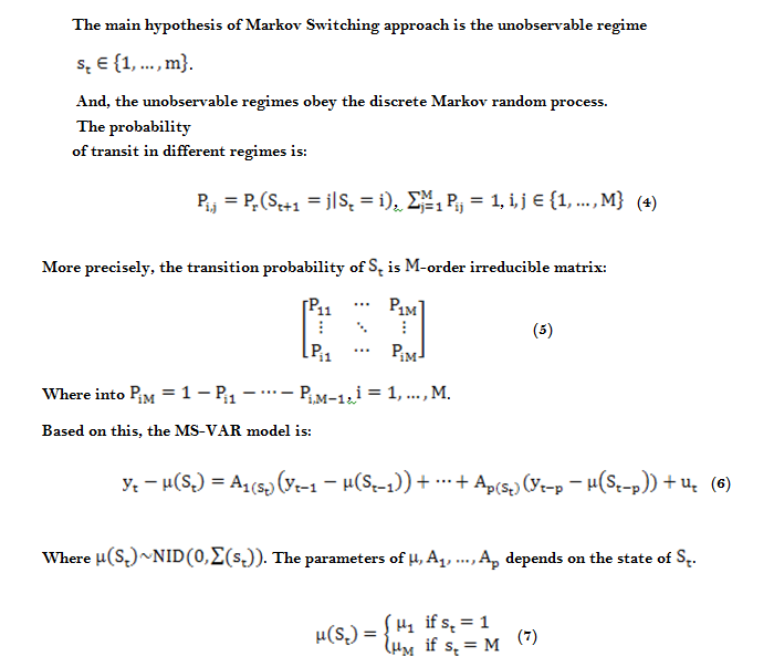
(A) Markov Switching Vector Auto-Regression Model
Hamilton (1989) firstly purpose the Markov Switching Vector Auto-regression (MS-VAR) model. The foundation of MS-VAR model is variables and economic state are the time-varying. Based on this condition, even if the variables are stationary, it is also inappropriate that the parameters in the model are not adjusted according by the economic state. The traditional model is set the relationship between variables is linear so that it cannot describe the potential non-linear relationship. Used the definition of “regime switching”, Hamilton (1989) contains the endogenous structural changes into the VAR model for capturing the time-varying state of macroeconomic and financial system. At present, the Markov-switching vector auto-regression (MS-VAR) model has been widely used in macroeconomic analysis about the various economic and financial series exhibit time varying behavior.
Compared with traditional VAR (p) model, MS-VAR model can shed light on the structure changes may exist in the data sample. It can be treated as the general form of linear VAR model. Considered a K-dimentional and lag P-order, time series vector
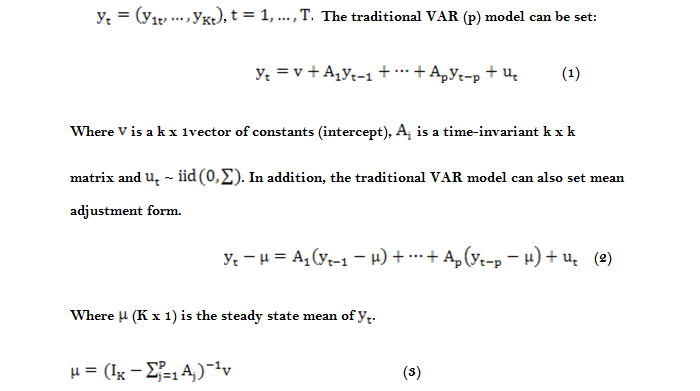
In addition, the MS-VAR model with intercept is:
![]()
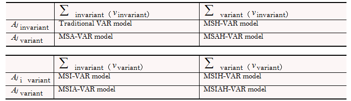
Markov switching vector auto-regression model has multiple types. Table 1 is the main types of MS-VAR model. I is the intercept term of Markov switching model. A represents the regression coefficient of Markov switching model. And, H is the heteroscedasticity of Markov switching model.
Table-1. Main Types of MS-VAR model
(A) Data Analysis
Having reviewed the exiting literature, there is a framework to analyse the asymmetric effects of China’s monetary policy on the stock market. Monetary policy uses quantity-based direct instruments and price-based indirect instruments to affect the stock market and macroeconomic development. The stock volume affects the money demand (Freidman, 1988) and the stock market uses the investment channel, wealth effects, and balance sheet channels to affect the macroeconomic development. The expected macroeconomic outlook affects the expected stock price and money supply. Based on this framework, this study uses the return rate of the Shanghai composite index, growth rate of GDP, growth rate of M2 and interest rate to shed light on the asymmetric effects of China’s monetary policy on the stock market. This study uses monthly data of China’s monetary policy, macroeconomy, and stock market from January 2003 to April 2015, complied by the data provider, Wind Database. Before 2003, China’s monetary policy gradually established monetary instruments, and after April 2015, China’s stock market has a structural break, causing it to experience a significant slowdown. To avoid the effects of a structural break, we used data from January 2003 to April 2015.
In the MS-VAR model, variables include growth rate of industrial added value, growth rate of M2, return rate of the Shanghai Composite Index, and the 7 day interbank weighted average interest rate. GDP could reflect the economy’s business cycle state. In this model, it is replaced by industry add value. The growth rate of industrial add value is adjusted for seasonal variations by the Census X12 method. This study uses quantity-based direct instruments and price-based indirect instruments to represent China’s monetary policy. M2 is the most important index of China’s quantity-based direct instruments. Considering the Chinese financial market, this study uses the 7-day interbank weighted average interest rate to reflect the supply and demand situation of money in the market. Table 2 shows the variables’ details and data source. Table 3 summarizes the descriptive statistics of these four variables in levels and first differences. Panel 1 shows the time series graphs of four variables in levels and first differences.
Table-2. Variables and Data source
| Variables | Details | Data source |
| RETURN | Return rate of Shanghai Composite Index | WIND Database |
| VA | Growth rate of Industrial added value | WIND Database |
| M2 | Growth rate of M2 | WIND Database |
| INTEREST | 7-day interbank weighted average interest rate | WIND Database |
Source From: Wind Database
Table-3. Descriptive Statistics of Variables
Panel A. Variables in levels
| Variables | obs | Mean | Median | Max | Min | Std | Skew | Kurt | JB | Prob |
| RETURN | 148 | 0.02935 | 0.00034 | 0.733267 | -0.358237 | 0.215195 | 0.732149 | 3.493201 | 14.7224 | 0.000635 |
| VA | 148 | 13.89689 | 14.7 | 22.5 | 5.4 | 4.184865 | -0.225537 | 1.989032 | 7.55739 | 0.022852 |
| INTEREST | 148 | 2.840909 | 2.565278 | 7.084358 | 0.99591 | 1.091019 | 0.738846 | 3.739323 | 16.83606 | 0.000221 |
| M2 | 148 | 16.98128 | 16.425 | 29.74 | 10.8 | 3.959658 | 1.403094 | 5.089234 | 75.47749 | 0 |
Panel B. Variables in first differences
| Variables | obs | Mean | Median | Max | Min | Std | Skew | Kurt | JB | Prob |
| DRETURN | 148 | 0.00082 | -0.030837 | 1.062086 | -0.857648 | 0.353596 | 0.668153 | 3.389739 | 11.86787 | 0.002648 |
| DVA | 148 | -0.116327 | -0.1 | 3.1 | -3.2 | 1.082529 | -0.230504 | 3.418377 | 2.373854 | 0.305158 |
| DINTEREST | 148 | 0.017212 | -0.0021 | 3.4404408 | -2.901897 | 0.658129 | 0.719215 | 10.42723 | 350.551 | 0.000000 |
| DM2 | 148 | -0.031973 | -0.1 | 5.03 | -3.02 | 1.127709 | 0.955339 | 6.278983 | 88.21484 | 0.000000 |
Notes: These two tables summarize descriptive statistics (sample mean, median, maximum, minimum, standard deviation, skewness, kurtosis, and the Jarque-Bera test statistics) of the return of the Shanghai Composite Index, growth rate of industrial add value, growth rate of M2, and the 7 day interbank weighted average interest rate. Figure 1 shows the descriptive statistics of the aforementioned variables measured in levels and in first differences. The sample period is from 2003.01 to 2015.04 and contains a total of 148 monthly observations.
(A) Variables in Levels
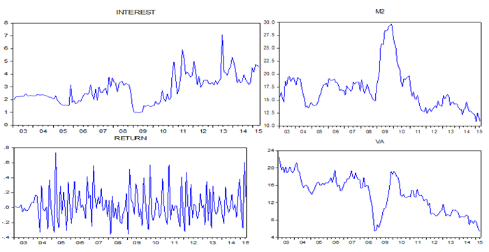
(B) Variables in first differences
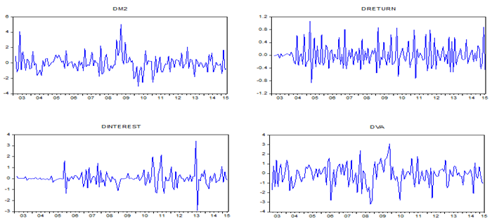
Figure-1. Time series graphs of four variables in levels and first differences
Table 4 summarizes the results of the unit root test. This study uses three different unit root tests, which are the Augmented Dickey Fuller (ADF) test, the Phillips-Perron (PP) test and the Zivot-Andrews (ZA) test. Using the time series plot of these four variables, we can judge the intercept and trend term in these four variables’ time series. It can be found that RETURN, VA, M2, and INTEREST have the intercept terms, but no trend terms. Therefore, the ADF test, PP test and the ZA test should include the intercept term and trend term. The results show that the level values of these four variables are stationary.
Table-4. Unit root test of variables in levels
| Unit root tests | ADF TEST | ZA TEST | PP TEST | ||||||
| Variables(C,T,K) | Obs | ADF Value | Pro. | CONS | BREAK | TREND | BREAK | PP Value | Pro. |
| RETURN(C,0,0) | 148 | -4.644311 | 0.0002 | -3.512112 | Sep-08 | -4.21512 | Jun-11 | -17.92118 | 0.000 |
| VA(C,0,0) | 148 | -17.35141 | 0 | -9.512211 | Nov-08 | -9.0102 | Jan-12 | -10.9662 | 0.000 |
| INTEREST(C,0,3) | 148 | -2.931156 | 0.0491 | -8.215125 | Feb-09 | -7.41512 | May-13 | -12.13172 | 0.000 |
| M2(C,0,2) | 148 | -3.681846 | 0.0053 | -3.212484 | Jun-07 | -5.341211 | Feb-14 | -3.363713 | 0.013 |
Note: This table summarizes the results of Augmented Dickey Fuller, the Phillips-Perron and Zivot-Andrews tests for a unit root. C means that intercept term. T is the trend term, which means that data has a long-term positive and negative trend. K expresses the lag order. The lag order is based on the AIC minimum criterion, which does not have autocorrelation and heteroscedasticity. The ZA test comprises a constant and a trend, while allowing for a single break in the constant and in both the constant (CONS) and the trend (TREND). The ZA test also provides the estimated break date (BREAK).
Table 5 summarizes the coefficient of pairwise correlations of the return rate of the Shanghai Composite index with industrial output, M2, and interest rate in the first difference. The results show that the correlation coefficients in the first differences of return of the Shanghai Composite with the growth rate of industrial add value, the growth rate of M2, and the 7 day interbank weighted average interest rate are respectively 0.01817, 0.03370, and -0.11825.
Table-5. Coefficients of correlation
| RETURN | VA | INTEREST | M2 | |
| RETURN | 1.00000 | 0.01817 | -0.11825 | 0.03370 |
| VA | 0.01817 | 1.00000 | -0.41952 | 0.35640 |
| INTEREST | -0.11825 | -0.41952 | 1.00000 | -0.62544 |
| M2 | 0.03370 | 0.35640 | -0.62544 | 1.00000 |
Notes: This table summarizes the Pearson coefficients among the dependent and exogenous variables. All variables are in first difference. The sample period is from 2003.01 to 2015.04 that contains a total of 148 monthly observations.
4. EMPIRICAL ANALYSIS AND DISCUSSION
Considered about the bull and bear markets have been explicitly identified by Maheu and McCurdy (2000); Pagan and Sossounov (2003); Edwards et al. (2003) and Lunde and Timmermann (2004). This study sets there are two regimes in the Markov Switching model.
Base on the principle of minimum criteria, this study uses the LR, FPE, AIC, SC, and HQ criteria to select the optimal number of lags. Using the Gauss package allows us to analyse the data and a variety of information to find the optimal lag. Table 6 shows that the lag orders of the VAR model is 2.
Table-6. Optimal Lag Orders
| Lag | LogL | LR | FPE | AIC | SC | HQ |
| 0 | -957.1137 | NA | 7.369085 | 13.34880 | 13.43130 | 13.38232 |
| 1 | -516.0803 | 851.4394 | 0.019735 | 7.425519 | 8.167972 | 7.727210 |
| 2 | -498.6374 | 32.70551 | 0.018071* | 7.333649* | 7.858034* | 7.613166* |
| 3 | -480.8295 | 32.40052 | 0.019272 | 7.400409 | 8.472842 | 7.836185 |
| 4 | -460.0227 | 36.70075* | 0.020124 | 7.445560 | 8.736061 | 7.903510 |
Notes: Using “*” represents the best lag in LR, FPE, AIC, SC, and HQ.
Compared with the value of LogL, the model should select the nonlinear model. Based on the minimum criteria of LR, FPE, AIC, SC, and HQ, table 7 shows that the model is MSIH (2)-VAR (2).
Table-7.Model Selection
| Lag | Linear model | Non-linear model | |||||
| VAR(2) | MSM(2)-VAR(2) | MSI(2)-VAR(2) | MSH(2)-VAR(2) | MSMH(2)-VAR(2) | MSIH(2)-VAR(2) | MSIAH(2)-VAR(2) | |
| LogL | -612.715 | -575.910 | -535.064 | -505.276 | -476.991 | -446. 06 |
-468.876 |
| LR | 119.5672 | 68.7754 | 73.9398 | 52.1832 | 20.46 6 |
26.7061* | 12.7942 |
| FPE | 0. 996 |
.2723 | 0.1736 | 0.1334 | 0.1339 | 0.1299* | 0.1490 |
| AIC | 9.1988 | 8.8647 | 8.4716 | 8.2399 | 8.2335 | 8.2129* | 8.3182 |
| SC | 9.5696 | 9.5322 | 9.7705 | 9.5009 | 10.0878 | 9.4358* | 10.4692 |
| HQ | 9.3495 | 9.1359 | 8.8634 | 8.8459 | 8.9870 | 8.7524* | 9.1923 |
Notes: The results are from the Gauss software package. M represents the mean term of the Markov state-dependent. I represents the intercept of Markov state-dependent. A indicates the auto-regressive parameter of Markov state-dependent. H indicates the error terms’ heteroscedasticity. Using “*” represents the best lag in LR, FPE, AIC, SC, and HQ.
Based on table 8, it can be found that regime 1 is the bull market. The coefficient of the four variables are positive. The switching probability reflects the possibility of converting between the stock market return rate and the industrial added value, broad monetary growth rates and interest rates in the different regimes. Based on the Table 9, it can be found that the probability of regime 1(2) switching to regime 2 (1) is 0.1808 (0.1814). The probability of the system staying in regime 1 (2) is 0.8192 (0.8186). Moreover, table 10 summarizes that regime 1 occupied the 65.49% of this system time. On average, it lasts 6.7498 months. Regime 2 occupied the 34.51% of the system time. Its average lasts 3.4211 months.
Table-8. The Results of MSIH (2)-VAR (2)
| Regime1 (Bull Market) | Regime2 (Bear Market) | |||||||
| Variables | Return | VA | Interest | M2 | Return | VA | Interest | M2 |
| RETURN(-1) | 0.6835** | 0.7686 ** | 0.0695 | 0.2205* | -0.2720* | 0.1446 | 0.4127 | -0.1040* |
| RETURN(-2) | 0.4530* | 1.2782 * | 0.2041 | 0.1541 | -0.1950 | -0.2779 | -0.2494 | -0.2068 |
Notes: The results are from the Gauss software package. According to the t-statistic value, “*” and “**” represent 5% and 1% significance level.
Table-9. Probability of Regime Switching
| Regime1 | Regime2 | |
| Regime1 | 0.8192 | 0.1808 |
| Regime2 | 0.1814 | 0.8186 |
Notes: The results are from the Gauss software package.
Table-10. Characteristics of Regimes
| Obs. | Pro. | Duration | |
| Regime1 | 96.9252 | 0.6549 | 6.7498 |
| Regime2 | 51.0748 | 0.3451 | 3.4211 |
Notes: The results are from the Gauss software package.
For the bull market state, it is mainly made up of two periods, which are from 2003 to 2006 and from 2012 to 2015. From 2003 to 2006, China’s economy had completely got rid of the adverse effects of the 1997 Southeast Asian Financial market. China’s stock market had attracted a large amount of domestic assets and international hot money. From 2012 to 2015, the People’s Bank of China issued the four-trillion stimulus plan and other unconventional monetary instruments to expand the money supply. China’s stock market in this period had recovered investors’ confidence. For the bear market state, from the main period was from 2007 to 2011. In this period, China’s economy and stock market were affected by the international financial crisis. Figure 2 shows the maps of each regimes’ probability.
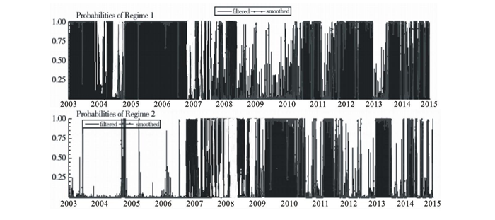
Figure-2. Maps of Probability of Regimes
Notes: Regimes in the China’s Shanghai Stock market. This figure identifies the Markov regimes (states), estimated using the MS-VAR model. Regime probabilities are given by the smoothed estimates (in solid black line).The regime 1 is the bull market state of Shanghai stock market. The bull market is from 2003 to 2006 and from 2012 to 2015. The regime 2 is the bear market state of Shanghai stock market. To the bear market, the main period was from 2007 to 2011.
4.1. Regime-Dependent Impulse Response Analysis
First, this study uses the impulse function to simulate the response of Shanghai Stock Market in the two regimes to China’s macroeconomic shock. The solid line shows the impulse response function. The result is reported in Figure 3. The horizontal axis represents retroactive periods. The vertical axis represents changes in China's stock markets.
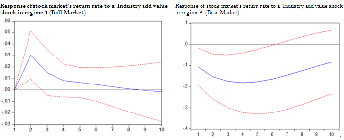
Figure-3. Industry of add value Impulse in Bull market and Bear market
Notes: This figure depicts the impulse response functions of the endogenous variables of the MS-VAR model in the bull market and bear market (Regime 1 and Regime 2). Estimated accumulated (10-periods ahead) IRFs to Industry of add value shock. The figure shows response to a positive one-standard-deviation shock in the Industry of add value. Lines with symbols stand for the upper and lower one standard error bands.
Figure 3 shows the results of China’s macroeconomic on the bull and bear market. In regime 1, the stock market is in the bull market state. Industry add value has significant and positive effects on the stock market. In the following periods, the effects of industry add value declines. In regime 2, the stock market is in the bear market. Industry add value has significant and negative effects on the stock market. Comparing the effects of industry add value in the bull market and bear market, the effects of industry add value in the bear market is more significant than in the bull market. It can be understood that the macroeconomy in a good situation cannot change the positive impact on the stock market in a bear market. Overall, China’s macroeconomic situation with the stock market has a dichotomy degree.
Moreover, this study uses the impulse function to simulate the response of Shanghai Stock Market in the two regimes to the China’s quantity-based direct monetary instrument shock. Used this impulse function aims to test the hypothesis 1. The solid line shows the impulse response function. The result is reported in Figure 4. The horizontal axis represents retroactive periods. The vertical axis represents changes in China's stock markets.
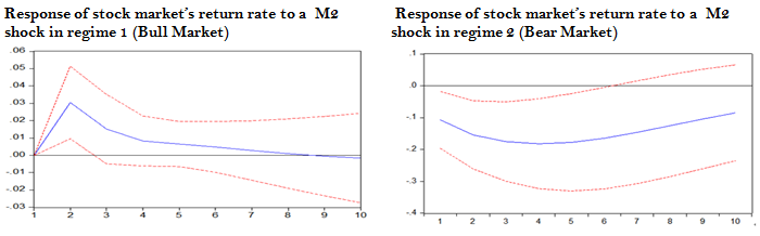
Figure-4. Quantity-Based Direct Monetary Instrument (M2) Impulse in the Bull market and Bear market
Notes: This figure depicts the generalized impulse response functions of the endogenous variables of the MS-VAR model in the bull market and bear market (Regime 1 and Regime 2). Estimated accumulated (10-periods ahead) IRFs to Quantity-Based Direct Monetary Instrument (M2) shock. The figure shows response to a positive one-standard-deviation shock in the Quantity-Based Direct Monetary Instrument (M2). Lines with symbols stand for the upper and lower one standard error bands.
Figure 4 shows the results of quantity-based direct instruments on the bull market and bear market. In the regime 1, stock market in the bull market. M2 has significant and positive effects on the stock market. In the following periods, the effects of M2 is declined. In the regime 2, stock market is in the bear market. M2 has significant and negative effects on the stock market. Based on this results, M2 has asymmetric effects on the stock market. Overall, the hypothesis 1 is true.
Furthermore, I use the impulse function to simulate the response of Shanghai Stock Market in the two regimes to China’s price-based indirect monetary instrument shock. This is for testing the hypothesis 2. The solid line shows the impulse response function. The result is reported in Figure 5. The horizontal axis represents retroactive periods. The vertical axis represents changes in China's stock markets.
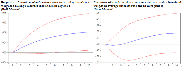
Figure-5. Price-Based Indirect Monetary Instrument (7-day interbank weighted average interest rate) Impulse in the Bull market and Bear market
Notes: This figure depicts the generalized impulse response functions of the endogenous variables of the MS-VAR model in the bull market and bear market (Regime 1 and Regime 2). Estimated accumulated (10-periods ahead) IRFs to Pirce-Based Indirect Monetary Instrument (M2) shock. The figure shows response to a positive one-standard-deviation shock in the Price-Based Indirect Monetary Instrument (7-day interbank weighted average interest rate). Lines with symbols stand for the upper and lower one standard error bands.
Figure 5 shows the results of price-based indirect monetary instrument on the bull market and bear market. The effects of the 7-day interbank weighted average interest rate on the stock market in the bull market state has a significant and positive effects on the stock market. To the bear market state, the effects of 7-day interbank weighted average interest rate on the stock market are not significant. It can be understood that 7-day interbank weighted average interest rate has asymmetric effects on the stock market. Overall, the hypothesis 2 is true. Moreover, the results from figure 6.3 to figure 6.4 show that both of quantity-based direct monetary instrument and price-based indirect monetary instrument have a stronger effects in a bull market than a bear market. The hypothesis 3 is false.
4.2. Robustness Checks
This study establishes a dynamic model of China’s monetary policy, macroeconomic and stock market. In order to ensure the accuracy of the results, this section uses the Shenzhen Stock Index to replace the Shanghai Composite Index to establish a new MS-VAR model. Figure 6 is the two regimes probability of Shenzhen Stock Exchange.
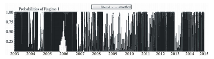
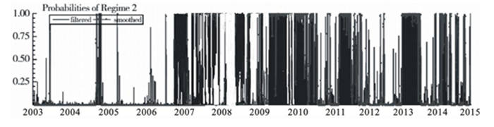
Figure-6. Maps of Probability of Regimes
Notes: Regimes in the China’s Shenzhen Stock market. This figure identifies the Markov regimes (states), estimated using the MS-VAR model. Regime probabilities are given by the smoothed estimates (in solid black line).The regime 1 is the bull market of Shenzhen stock market. The bull market is from 2003 to 2006 and from 2012 to 2015. The regime 2 is the bear market of Shenzhen Stock Market. To the bear market, the main period was from 2007 to 2010.
This part uses the impulse function to simulate the response of Shenzhen Stock Market in the two regimes to the shock of China’s macroeconomy, quantity-based direct monetary instrument and price-based indirect monetary instrument. The solid line shows the impulse response function. The results are reported from figure 6.6 to figure 6.8. The horizontal axis represents retroactive periods. The vertical axis represents changes in China's stock markets. From Figure 7 to Figure 9, the results show that the quantity-based direct instruments and price-base indirect instruments of China’s monetary policy have asymmetric effects on the bull market and bear market of Shenzhen stock market. These results are similar with the Shanghai stock market.
Figure-7. Industry of add value Impulse in Bull market and Bear market
Notes: This figure depicts the generalized impulse response functions of the endogenous variables of the MS-VAR model in the bull market and bear market (Regime 1 and Regime 2). Estimated accumulated (10-periods ahead) IRFs to Industry of add value shock. The figure shows response to a positive one-standard-deviation shock in the Industry of add value. Lines with symbols stand for the upper and lower one standard error bands.
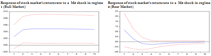
Figure-8. Quantity-Based Direct Instruments (M2) Impulse in the Bull market and Bear market
Notes: This figure depicts the generalized impulse response functions of the endogenous variables of the MS-VAR model in the bull market and bear market (Regime 1 and Regime 2). Estimated accumulated (10-periods ahead) IRFs to Quantity-Based Direct Monetary Instrument (M2) shock. The figure shows response to a positive one-standard-deviation shock in the Quantity-Based Direct Monetary Instrument (M2). Lines with symbols stand for the upper and lower one standard error bands.
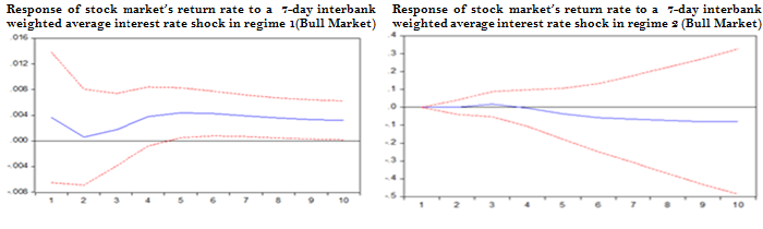
Figure-9. Price-Based Indirect Instruments (7-day interbank weighted average interest rate) Impulse in the Bull market and Bear market
Notes: This figure depicts the generalized impulse response functions of the endogenous variables of the MS-VAR model in the bull market and bear market (Regime 1 and Regime 2). Estimated accumulated (10-periods ahead) IRFs to Pirce-Based Indirect Monetary Instrument (7-day interbank weighted average interest rate) shock. The figure shows response to a positive one-standard-deviation shock in the Price-Based Indirect Monetary Instrument (7-day interbank weighted average interest rate). Lines with symbols stand for the upper and lower one standard error bands.
In a summary, using the above MS-VAR model, this study has tested the three hypotheses. First, results indicate that quantity-based direct monetary instrument has asymmetric effects on China’s stock market in a bull market and a bear market. This result certificates that the hypothesis 1 is true. Second, price-based direct monetary instrument has asymmetric effects on China’s stock market in a bull market and a bear market. This result certificates that the hypothesis 2 is true. To the hypothesis 3, the results show that the effects of quantity-based direct monetary instrument on the stock market in a bull market are stronger than a bear market. The hypothesis 3 is false.
5. CONCLUSIONS AND RECOMMENDATIONS
This study establishes a Markov Switching vector auto-regression (MS-VAR) model to shed light on the dynamic relationship between China’s monetary policy, macroeconomy, and stock market since January 2003 to April 2015. Through the construction of the model and data analysis, this study makes the following conclusions. First, the results show that there exists a significant non-linear relationship between China’s monetary policy, macroeconomy and stock market from January 2003 to April 2015. Second, from January 2003 to April 2015, China’s monetary policy has asymmetric effects on the stock market. To the quantity-based direct monetary instrument, M2 has significant and positive effects on the stock market in the bull market. But, in the bear market, M2 has significant and negative effects. Turning to the price-based indirect monetary instrument, the effect of the 7-day interbank weighted average interest rate on the stock market in the bull market is significant and positive. In the bear market, the effects of 7-day interbank weighted average interest rate on the stock market are not significant. Third, the effects of China’s monetary policy on the stock market in the bull market are stronger than the bear market. This result is different with Chulia et al. (2010) and Jansen and Tsai (2010). The reason of this result can be explained China’s stock market in the bear market has completely lost financial institutions and investors’ confidences. Fourth, from January 2003 to April 2015, China's macroeconomy and stock market presents a dichotomy. This result is similar with that of. Affected by the 2008 international financial crisis, China’s economy has downside risks. After the People’s Bank of China adopted a series of expansionary monetary policy, China's economy stabilised to pick up in the first quarter of 2009. However, China’s stock market entered a downturn since the second half of 2009. Based on the above analysis, this study draws some recommendations to China’s policymakers. First, this study suggests that policymakers need to accelerate the reform of the stock market; that is, to a certain extent, the authorities could enhance the flexibility and autonomy of China’s listed companies. Second, China should gradually reduce the leading role of state-owner assets in the stock market. Third, policymakers should furtherly strengthen the effects of price-based indirect monetary instruments on the stock market.
| Funding: This study received no specific financial support. |
| Competing Interests: The authors declare that they have no competing interests. |
| Contributors/Acknowledgement: Both authors contributed equally to the conception and design of the study. |
REFERENCES
Airaudo, M., R. Cardani and K. Lansing, 2011. Monetary policy and asset prices with belief-driven fluctuations and news shocks. Philadelphia, PA: LeBow College of Business, Drexel University. Retrieved from http://www.be.wvu.edu/econ_seminar/documents/11-12/airaudo.pdf .
Almeida, H. and M. Campello, 2007. Financial constraints, assets tangibility, and corporate investment. Review of Financial Studies, 20(5): 1429-1460. View at Google Scholar | View at Publisher
Andersen, T.G., T. Bollerslev, F.X. Diebold and C. Vega, 2007. Real-time price discovery in global stock, bond and foreign exchange markets. Journal of International Economics, 73(2): 251–277. View at Google Scholar | View at Publisher
Basistha, A. and A. Kurov, 2008. Macroeconomic cycles and the stock market’s reaction to monetary policy. Journal of Banking and Finance, 32(12): 2606–2616. View at Google Scholar | View at Publisher
Berkman, N. G., 1978. On the significance of weekly changes in M1. New England Economic Review, 78(1798): 5-22. View at Google Scholar
Bernanke, B. S. and K. N. Kutter, 2005. What explains the stock market's reaction to federal reserve policy? Journal of Finance, 60(3): 1221-1257. View at Google Scholar | View at Publisher
Bernanke, B.S. and R.R. Vincent, 2004. Conducting monetary policy at very low short-term interest rates. American Economic Review, 94(2): 85-90. View at Google Scholar | View at Publisher
Brandley, M.D. and D.W. Jansen, 2004. Forecasting with a nonlinear dynamic model of stock returns and industrial production. International Journal of Forecasting, 20(2): 321-342. View at Google Scholar | View at Publisher
Carlos, T., 2008. Search and matching frictions and optimal monetary policy. Journal of Monetary Economics, 55(5): 936-956.View at Google Scholar | View at Publisher
Castelnuovo, E. and S. Nistico, 2010. Stock market conditions and monetary policy in a DSGE model for the U.S. Journal of Economic Dynamics and Control, 34(9): 1700-1731. View at Google Scholar | View at Publisher
Chen, S.S., 2007. Does monetary policy has asymmetric effects on stock returns? Journal of Money, Credit, and Banking, 39(2-3): 677-688. View at Google Scholar | View at Publisher
Chulia, H., M. Martens and D. van Dijk, 2010. Asymmetric effects of federal funds target rate changes on S&P100 stock returns, volatilities and correlations. Journal of Banking and Finance, 34(4): 834-839. View at Google Scholar | View at Publisher
Cook, T. and T. Hahn, 1989. The effect of changes in the federal funds rate target on market interest rates in the 1970s. Journal of Monetary Economics, 24(3): 331-351.View at Google Scholar | View at Publisher
Cooper, R.M., 1974. The control of eye fixation by the meaning of spoken language: A new methodology for the real-time investigation of speech perception, memory, and language processing. Cognitive Psychology, 6(1): 84-107.View at Google Scholar | View at Publisher
Cover, J.P., 1992. Asymmetric effects of positive and negative money-supply shocks. Quarterly Journal of Economics, 107(4): 1261–1282. View at Google Scholar | View at Publisher
DeLong and Summers, 1988. How does macroeconomic policy matter? Brookings Papers on Economic Activity. pp: 433-480.
Edwards, S., G.B. Javier and P.d.G. Fernando, 2003. Stock market cycles, financial liberalization and volatility. Journal of International Money and Finance, 22(7): 925–955. View at Google Scholar | View at Publisher
Freidman, M., 1988. Money and the stock market. Journal of Political Economy, 96(2): 221-245. View at Google Scholar
Funke, M., M. Paetz and E. Pytlarczyk, 2011. Stock market wealth effects in an estimated DSGE model for Hong Kong. Economic Modelling, 28(1-2): 316 -334.View at Google Scholar | View at Publisher
Garcia, R. and H. Schaller, 1995. Are the effects of monetary policy asymmetric? Working Paper No. 95-6, Department of Economics. University of Montreal.
Giorgio, D.G. and S. Nistico, 2007. Monetary policy and stock prices in an open economy. Journal of Money, Credit and Banking, Blackwdl Publishing, 39(8): 1947-1985. View at Google Scholar | View at Publisher
Guo and Li, 2004. Empirical analysis the relationship between Chinese stock market and monetary policy. Journal of Econometrics Research, 6: 18-27.
Guo, F., J. Hu and M. Jiang, 2013. Monetary shocks and asymmetric effects in an emerging stock market: The case of China. Economic Modelling, 32(C): 532-538.View at Google Scholar | View at Publisher
Hamburger, M.J. and L.A. Kochin, 1971. Money and stock prices: The channels of influences. Journal of Finance, 27(2): 231-249.
Hamilton, J.D., 1989. A new approach to the economic analysis of nonstationary time series and the business cycle. Econometrica, Econometric Society, 57(2): 357–384. View at Google Scholar | View at Publisher
Homa, K.E. and D.M. Jaffee, 1971. The supply of money and common stock prices. Journal of Finance, 26(5): 1045-1066. View at Google Scholar | View at Publisher
Hyde, S. and D. Bredin, 2005. Regime changes in the relationship between stock returns and macro economy. SSRN Working Paper, No. 35.
Jansen, D. and C. Tsai, 2010. Monetary policy and stock returns: Financing constraints and asymmetries in bull and bear markets. Journal of Empirical Finance, 17(5): 981-990. View at Google Scholar | View at Publisher
Keran, M.W., 1971. Expectation, money and the stock market. Federal Reserve Bank of St. Louis Review, 53: 16-31.
Konrad, E., 2009. The impact of monetary policy surprises on asset return volatility: The case of Germany. Financial Markets and Portfolio Management, 23(2): 111–135. View at Google Scholar | View at Publisher
Kurov, A., 2010. Investor sentiment and the stock market’s reaction to monetary policy. Journal of Banking and Finance, 34(1): 139-149. View at Google Scholar | View at Publisher
Livdan, D., H. Sapriza and L. Zhang, 2009. Financially constrained stock returns. Journal of Finance, 64(4): 1827-1862. View at Google Scholar | View at Publisher
Lobo, B.J., 2002. Interest rate surprises and stock prices. Financial Review, 37(1): 73-91 View at Google Scholar | View at Publisher
Lunde, A. and A.G. Timmermann, 2004. Duration dependence in stock prices: An analysis of bull and bear markets. Journal of Business and Economic Statistics, 22(3): 253–273. View at Google Scholar | View at Publisher
Lynge, M. J., 1981. Money supply announcements and stock prices. Journal of Portfolio Management, 8(1): 40-43.View at Google Scholar
Maheu, J.M. and T.H. McCurdy, 2000. Identifying bull and bear markets in stock returns. Journal of Business and Economic Statistics, 18(1): 100–112. View at Google Scholar | View at Publisher
Milani, F., 2008. Learning about the interdependence between the macro-economy and the stock market [EB]. Mimeo: University of California at Irvine.
Milani, F., 2011. The impact of foreign stock markets on macroeconomic dynamics in open economies: A structural estimation. Journal of International Money and Finance, 30(1): 111-129.View at Google Scholar | View at Publisher
Nistico, S., 2005. Monetary policy and stock price dynamics in a DSGE framework [EB]. LUISS Lab on European Economics (LLEC), Working Paper, No. 28.
Pagan, A.R. and K.A. Sossounov, 2003. A simple framework for analysing bull and bear markets. Journal of Applied Econometrics, 18(1): 23–46. View at Google Scholar | View at Publisher
Piergallini, A., 2004. Real balance eects, determinacy and optimal monetary policy. Economic Inquiry, 44(3): 497-511.
Piergallini, A., 2006. Real balance effects and monetary policy. Economic Inquiry, 44(3): 497-511.View at Google Scholar | View at Publisher
Qian Y. and G. Roland, 1988. Federalism and the soft budget constraint. American Economic Review, 88(5): 1143-1162.
Rigobon, R. and B. Sack, 2001. Measuring the reaction of monetary policy to the stock market. Cambridge: National Bureau of Economic Research.
Rozeff, 1974. Money and stock prices: Market efficiency and the lag in effect of monetary policy. Journal of Financial Economics, 1(3): 245-302. View at Google Scholar
Sellin, P., 2001. Monetary policy and the stock market: Theory and empirical evidence. Journal of Economic Surveys, 15(4): 491-541. View at Google Scholar | View at Publisher
Sensier, D.R. Osborn and N. Öcal, 2002. Asymmetric interest rate effects for the UK real economy, Centre for Growth and Business Cycle Research Discussion Paper Series 10, Economics, The Univeristy of Manchester.
Smirlock M. and J. Yawitz, 1985. Asset returns, discount rate changes, and market efficiency. Journal of Finance, 40(4): 1141-1158.View at Google Scholar | View at Publisher
Sprinkel, B.W., 1964. Money and stock prices. Homewood, Ill: Richard D. Irwin, Inc.
Thorbecke, W., 1997. On stock market returns and monetary policy. Journal of Finance, 52(2): 635-654. View at Google Scholar | View at Publisher
Weise, C.L., 1999. The asymmetric effects of monetary policy: A nonlinear vector auto-regression approach. Journal of Money, Credit and Banking, 31(1): 85-108. View at Google Scholar | View at Publisher
Zare, R., M. Azali and M.S. Habibullah, 2013. Monetary policy and stock market volatility in the ASEAN5: Asymmetries over bull and bear markets. Procedia Economics and Finance, 7: 18-27. View at Google Scholar | View at Publisher
Zhang, X.Z., Z.Y. Liu and J. Wang, 2010. Dual effects of monetary policy on corporate investment. Journal of Manage Sciences, 5: 108-119.