DOES PRICING DEVIATION OF EXCHANGE-TRADED FUNDS PREDICT ETF RETURNS?

Jung-Chu Lin

Associate Professor, Department of Banking and Finance, Takming University of Science and Technology, Taipei, Taiwan

Keywords:Exchange-traded fund, Pricing deviation, ETF return, ETF pricing efficiency, Creation-redemption process, Arbitrage strategy

ARTICLE HISTORY: Received:13 April 2017Revised:10 May 2017 Accepted:5 June 2017Published:19 June 2017

Contribution/ Originality:: This study contributes the first logical analysis which classifies ETFs into four types to investigate whether inactive ETFs’ pricing deviation can predict future ETF returns better than active ETFs’. The results demonstrate that inactive ETFs’ pricing deviation does predict future ETF returns better and longer.

1. INTRODUCTION

Even though exchange traded funds (ETFs) resemble closed-end funds (CEFs) in many facets, ETFs have a unique feature that additional shares can be created and redeemed by investors through authorized dealers (Engle and Sarkar, 2006). The creation–redemption process allows investors to engage in an arbitrage strategy that adjusts the supply of ETF shares on the market, and thus helps ETF shares to trade at prices approximating the calculated net asset value (NAV) of the underlying portfolio (the underlying value). However, because the creation–redemption mechanism requires a minimum shares for each creation or redemption order (i.e., a creation and redemption unit), the arbitrage trading on ETFs with poor marketability may not be able to be executed smoothly and instantaneously. The deviation (pricing error) between the NAVs and market prices of these less marketable ETFs may be therefore much larger and mostly negative when compared with that of actively traded ETFs. Using actively traded ETFs as a benchmark, this article investigates the extent and properties of the less marketable ETFs’ pricing errors (premiums or discounts), how their NAVs and market prices lead each other, and whether their pricing errors can predict near-term returns better.

Taiwan currently has 13 domestic-component-security ETFs trading on the Taiwan Stock Exchange Corporation (TWSE), since the 2003 launch of the first ETF. While nine of the 13 ETFs have correspondent futures trading on the Taiwan Futures Exchange for their underlying indexes, only three of them have average daily share turnover that are greater than their corresponding creation and redemption unit during the data period August 31, 2006 to June 30, 2016. This study defines those ETFs with an average daily share turnover greater than their creation and redemption unit as active ETFs and the opposites as inactive ETFs. Further considering the existence of corresponding futures for the underlying indexes may affect the ETF pricing efficiency, this study divides the 13 ETFs into four types: (1) active ETFs that have futures markets for the underlying indexes; (2) active ETFs that do not have corresponding futures for the underlying indexes; (3) inactive ETFs that have corresponding index futures; and (4) inactive ETFs that do not have corresponding index futures. This paper compares the four different types of ETFs in terms of pricing errors, lead-lag relationship between NAVs and market prices and the ability of the pricing deviation to predict ETF near-term returns.

2. LITERATURE AND HYPOTHESES

A vast literature shows that CEF share prices generally trade at a substantial and long-lasting discount to the NAV. Explanations for the CEF discount include unrealized capital gains tax (Malkiel, 1977) portfolio illiquidity (Deli and Varma, 2002; Cherkes et al., 2009) managerial performance (Chay and Trzcinka, 1999; Berk and Stanton, 2007) agency costs (Barclay et al., 1993; Coles et al., 2000) and distribution policies (Johnson et al., 2006; Wang and Nanda, 2011). Investors who notice any discrepancy between the NAV and the fair market value have the opportunity to make a profit by buying at a discount and selling at a premium (Chalmers et al., 2001; Goetzmann et al., 2001; Boudoukh et al., 2002). Yet not until the development of the ETF creation and redemption mechanism are the arbitrage opportunities really exploited profitably. The creation and redemption process for ETFs allows arbitrage strategies to be executed effectively whenever the share prices deviate from the underlying value. If the creation–redemption process works efficiently, ETF shares should not trade at significant deviation from the fair value of the portfolio (Engle and Sarkar, 2006). The lower marketability in those inactive ETFs on the TWSE may block the efficient work of the creation–redemption process, making inactive ETF shares trade at significant deviation from the underlying value. For inactive ETFs, the bi-directional lead-lag relationship between NAVs and market prices of active ETFs, found in Lin (2011) may become a one-way lead-lag relationship that only NAVs lead market prices. However, having corresponding futures markets for the underlying indexes may improve the pricing efficiency and the connection between NAVs and market prices of inactive ETFs. Therefore, this paper develops three hypotheses to test as follows:

1. This paper expects inactive ETFs, like CEFs, trade at a substantial and mostly-negative pricing error to the NAV. The distribution of their pricing errors is expected to be more skewed to the right and have a higher proportion for the negative than active ETFs. However, if an inactive ETF has corresponding futures for its underlying index, the deviation and the skewness to the right may shrink.
2. While active ETFs generally display a bi-directional lead-lag relationship between NAVs and market prices, this paper expects a one-way lead-lag relationship for inactive ETFs where only NAVs lead market prices. However, if an inactive ETF has corresponding futures for its underlying indexes, this one-way lead-lag relationship may evolve into a bi-directional one that the market price also leads the NAV; that is, the creation–redemption process may work more effectively to enhance the connection between the market price and the NAV.
3. Since the arbitrage on the pricing deviation of inactive ETFs needs more time (days) to accumulate enough shares for satisfying the requirement of the creation and redemption unit, the pricing errors of inactive ETFs may predict ETFs’ near-term returns better and longer.  

3. DATA AND DESCRIPTIVE STATISTICS

All the 13 ETFs, composed of the listed shares on TWSE, are included in the sample of this study. To identify the type of each ETF, I collect relevant information of the 13 ETFs summarized in Table 1, and categorize all these ETFs to one of the four types of ETFs as shown in Table 2. 

Table-1. The 13 ETFs with domestic component securities on the TWSE

Note: One lot equals 1,000 shares. Average daily share turnovers are computed using daily data between August 31, 2006 and June 30, 2016. “Y” indicates the ETF has corresponding index futures on the market, while “N” means the ETF does not have corresponding index futures.
Source: the TWSE.

Table-2. Classification of the 13 ETFs

Source: the Taiwan Futures Exchange and this study.

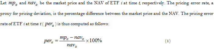
This study gathers daily data of the market price and the NAV of the 13 ETFs between August 31, 2006 and June 30, 2016 from the Taiwan Economic Journal (TEJ) database to compute the pricing error rates of the 13 ETFs of this data period. The movements of the pricing error rates for the four types of ETFs during this data period are plotted in Fig. 1 and the descriptive statistics of each ETF by types are presented in Table 3. For comparison purposes, the vertical axes of the four panels in Fig. 1 have the same maximum, minimum and spacing for the scale.

Fig. 1 shows that inactive ETFs do have a larger-extent and more volatile pricing error than active ETFs. In particular, the inactive ETFs without corresponding index futures seem to have the largest-magnitude pricing error, and the volatility of their pricing errors seems the greatest. In addition to supporting the findings in Fig. 1, Table 3 shows that the distribution of pricing error rates of inactive ETFs are more skewed to the right and that their proportions of the negative pricing error are higher than those of active ETFs. All these results support the expectations of hypotheses (1) that inactive ETFs trade at a substantial and mostly-negative deviation to the NAV and that the existence of corresponding index futures does mitigate the deviation.

Fig-1. Pricing error rates of the four types of ETFs, August 31, 2006 to June 30, 2016.

Source: the TEJ database.

Table-3. Descriptive statistics of the four types, 13 ETFs’ pricing error rates, August 31, 2006 to June 30, 2016

Source: The TEJ database and this study.

4. METHODOLOGY AND EMPIRICAL RESULTS

I first use the vector autoregression (VAR) to model the dynamic relationship between the NAV and the market price of each ETF. Through this model specification, I use Schwarz information criterion to decide the optimum lag length for each ETF’s NAV and market price relationship. Then I use the decided optimum lag length to execute the Granger Causality test to examining the causation between the NAV and the market price of each ETF. The results, presented in Table 4, show that the longest optimum lag length is 4 and that the length seems independent of ETF type. For all the 13 ETFs, the NAV does Granger cause the market price, yet only the active ETFs with corresponding index futures and some of the inactive ETFs with corresponding index futures display the reverse lead-lag relationship, i.e. the market price Granger causes the NAV. These results support the expectations of hypotheses (2) that inactive ETFs mostly have a one-way lead-lag relationship, compared to active ETFs. However, if an inactive ETF has corresponding futures for its underlying indexes, this one-way lead-lag relationship may evolve into a bi-directional one that the market price also leads the NAV.

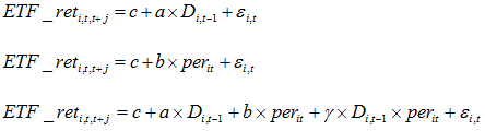
Since all the NAV and market price series are non-stationary, I further test the presence of cointegrating relationship between each ETF’s NAV and market price. The results show that each ETF’s NAV and market price do have a cointegrating relationship between them. The properties of each cointegration equation (CE) are presented in Table 4. To investigate the ability of ETF pricing deviation to predict subsequent ETF returns, this paper constructs three testing equations as follows:

Table-4. The causality and cointegration relationship between NAVs and market prices of the 13 ETFs

Note: The optimum lag lengths are selected by Schwarz information criterion. The results of the Granger causality test are reported by F-statistics and their p-values in the parentheses. Johansen cointegration tests and Schwarz criteria are applied to decide whether NAVs and market prices are cointegrated and which type their cointegration relationship (cointegration equation, CE) is. *, ** and *** indicate significance at the 10%, 5% and 1% levels, respectively.

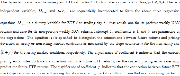
The regression results, presented in Table 5, show that all the four-type ETFs’ pricing deviation is significantly and negatively related to one-day future ETF returns, indicating that a discount in ETF pricing predicts one-day future positive returns and vice versa. However, only inactive ETFs have pricing deviation significantly and negatively related to two- to four-day future ETF returns, supporting the hypothesis (3) that the pricing errors of inactive ETFs may predict ETF returns better and longer. In a few cases, the connection between future ETF market price returns and current pricing deviation in a rising market is stronger than that in a non-rising market.

Table-5. Regression results based on various-period future ETF returns against the market condition dummy and the pricing errors rates

Note: The panel reports estimates from the OLS regressions of one-day future ETF returns on the dummy variable for market condition and the pricing error rate. Robust p-values following White or Newey and West (1987) corrected t-statistics with optimum lag length are reported in parentheses. *, ** and *** indicate significance at the 10%, 5% and 1% levels, respectively. The sample period is from August 31, 2006 through June 30, 2016.

Note: The panel reports estimates from the OLS regressions of two-day future ETF returns on the dummy variable for market condition and the pricing error rate. Robust p-values following White or Newey and West (1987) corrected t-statistics with optimum lag length are reported in parentheses. *, ** and *** indicate significance at the 10%, 5% and 1% levels, respectively. The sample period is from August 31, 2006 through June 30, 2016.

Note: The panel reports estimates from the OLS regressions of three-day future ETF returns on the dummy variable for market condition and the pricing error rate. Robust p-values following White or Newey and West (1987) corrected t-statistics with optimum lag length are reported in parentheses. *, ** and *** indicate significance at the 10%, 5% and 1% levels, respectively. The sample period is from August 31, 2006 through June 30, 2016.

Note: The panel reports estimates from the OLS regressions of four-day future ETF returns on the dummy variable for market condition and the pricing error rate. Robust p-values following White or Newey and West (1987) corrected t-statistics with optimum lag length are reported in parentheses. *, ** and *** indicate significance at the 10%, 5% and 1% levels, respectively. The sample period is from August 31, 2006 through June 30, 2016.

5. CONCLUSION

This study examines whether the poor marketability of inactive ETFs block the efficient work of the creation-redemption process, making their pricing deviation, lead-lag relationship between the NAVs and market prices and ability to predict future ETF returns distinct from those of active ETFs. The empirical results show that inactive ETFs do trade at a substantial, more volatile and mostly negative pricing deviation to the NAV and that the existence of corresponding index futures trading may mitigate the deviation and improve the pricing efficiency. While active ETFs display a bi-directional lead-lag relationship between NAVs and market prices, most of the inactive ETFs only display a one-way lead-lag relationship, i.e. only NAVs Granger cause market prices. However, if an inactive ETF has corresponding futures market for its underlying index, the pricing deviation may shrink and the one-way lead-lag relationship may evolve into a bi-directional one that market prices also lead NAVs. Finally, the regression results show that both active and inactive ETFs’ pricing deviation relates significantly and negatively to one-day future ETF returns, indicating that a discount in ETF may predict a positive one-day future return and a premium predict a negative return. However, only inactive ETFs’ pricing deviation relates significantly and negatively to longer-day future ETF returns, indicating that since the arbitrage on the pricing deviation of inactive ETFs needs more days to accumulate enough shares for satisfying the requirement of the creation and redemption unit, their deviation may predict ETF returns better and longer.

REFERENCES

Barclay, M., C. Holderness and J. Pontiff, 1993. Private benefits from block ownership and discounts on closed-end funds. Journal of Financial Economics, 33(3): 263–291. View at Google Scholar | View at Publisher

Berk, J.B. and R. Stanton, 2007. Managerial ability, compensation, and the closed-end fund discount. Journal of Finance, 62(2): 529–556. View at Google Scholar | View at Publisher

Boudoukh, J., M. Richardson, M. Subrahmanyam and R. Whitelaw, 2002. Stale prices and strategies for trading mutual funds. Financial Analysts Journal, 58(4): 53–71. View at Google Scholar | View at Publisher

Chalmers, J., R. Edelen and G. Kadlec, 2001. On the perils of financial intermediaries setting security prices: The mutual fund wild card option. Journal of Finance, 56(6): 2209–2236. View at Google Scholar | View at Publisher

Chay, J.B. and C. Trzcinka, 1999. Managerial performance and the cross-sectional pricing of closed-end funds. Journal of Financial Economics, 52(3): 379–408. View at Google Scholar | View at Publisher

Cherkes, M., J. Sagi and R. Stanton, 2009. A liquidity-based theory of closed-end funds. Review of Financial Studies, 22(1): 257–297. View at Google Scholar | View at Publisher

Coles, J., J. Suay and D. Woodbury, 2000. Fund advisor compensation and closed-end funds. Journal of Finance, 55(3): 1385–1414. View at Google Scholar | View at Publisher

Deli, D. and R. Varma, 2002. Closed-end versus open-end: The choice of organizational form. Journal of Corporate, 8(1): 1–27. View at Google Scholar | View at Publisher

Engle, R. and D. Sarkar, 2006. Premiums-discounts and exchange traded funds. Journal of Derivatives, 13(4): 27–45. View at Google Scholar 

Goetzmann, W., Z. Ivkovic and G. Rouwenhorst, 2001. Day trading international mutual funds: Evidence and policy solutions. Journal of Financial and Quantitative Analysis, 36(3): 287–309. View at Google Scholar | View at Publisher

Johnson, S., J. Lin and K. Song, 2006. Dividend policy, signaling, and discounts on closed-end funds. Journal of Financial Economics, 81(3): 539–562. View at Google Scholar | View at Publisher

Lin, J.C., 2011. Which is dominant? ETFs or highly capitalized stocks: Evidence from an emerging market. International Review of Business Research Papers, 2(1): 90-105. View at Google Scholar 

Malkiel, B.G., 1977. The valuation of closed-end investment company shares. Journal of Finance, 32(3): 847–859. View at Google Scholar | View at Publisher

Newey, W.K. and K.D. West, 1987. A simple, positive semi-definite, heteroskedasticity and autocorrelation consistent covariance matrix. Econometrica, 55(3): 703-708. View at Google Scholar | View at Publisher

Wang, Z.J. and V. Nanda, 2011. Payout policies and closed-end fund discounts: Signaling, agency costs, and the role of institutional investors. Journal of Financial Intermediation 20(4): 589-619. View at Google Scholar | View at Publisher