ESTIMATING AIR PARTICULATE MATTER 10 USING LANDSAT MULTI-TEMPORAL DATA AND ANALYZING ITS ANNUAL TEMPORAL PATTERN OVER GAZA STRIP, PALESTINE

Abdallah Shaheen¹⁺ --- Aqeel Ahmed Kidwai² --- Noor Ul Ain³ --- Midyan Aldabash⁴ --- Aatif Zeeshan⁵

^1,3,5Researcher, Department of Meteorology, COMSATS Institute of Information Technology, Islamabad, Pakistan

²Principal Scientific Officer, Department of Meteorology, COMSATS Institute of Information Technology, Islamabad, Pakistan

⁴PhD Researcher, Geomatics Engineering Department, Istanbul Teknik Üniversitesi İnşaat Fakültesi, Istanbul, Turkey

Keywords: PM10, TM, ETM+, Atmospheric reflectance, Gaza strip, Urbanization.

Article History: Received: 16 January 2017, Revised: 10 February 2017, Accepted: 22 February 2017, Published: 3 March 2017

Contribution/ Originality: The paper contributes the first ever research on the air quality of Gaza Strip, Palestine. The propose algorithm in this research is to estimate the particulate matter 10 using remote sensing data and also study the impact of environmental parameters on air quality during last 15 years in the study area.

1. INTRODUCTION

The addition of foreign fine particles into the atmosphere gives rise to air pollution, especially when the particles originate from hazardous sources. It basically, is a mixture of solid, liquid and gaseous particles. Air pollution is caused when these particles inhabit the atmosphere in an elevated amount, menacing to human health by increasing disease risks and/or destroying the cultural patrimony in urbanized areas. The core factor behind the air pollution is ever increasing human-induced anthropogenic activities such as vehicle emissions, industry and urbanization loading a huge amount of smoke and other harmful gases into the atmosphere. Motor traffic emissions are one of the most important sources for air pollution across the globe. Pollutant particles are dispersed and diluted during emission and also exhibit photochemical reactions [1].

Air pollution shows adverse effects on human health [2, 3] as well as atmospheric visibility [4, 5] and climate change [6]. Chemical particles like sulfur dioxide (SO₂), nitrogen oxide (NOx), carbon monoxide (CO), heavy metallic compounds and Suspended particulate matters (SPM) are responsible for acute and chronic lung diseases, heart diseases; and also cause the aggravation of existing lung diseases such as bronchitis and asthma. Thus, affecting the average human life expectancy rate [7, 8].

PM10 consists of fine solid particulates along with very small water droplets present in the air, ranging to a size of less than 10 microns. PM10 is generally divided into fine particulates with size smaller than 2.5 microns i.e. PM2.5, and courser particulates lesser than 10 microns i.e. PM 10. National Ambient Air Quality Objectives for Particulate Matter [9] categorized PM10 into two divisions, i.e. primary particles (sea salt, minerals and carbonaceous compounds) and secondary particles (those which have been created in the atmosphere by the interaction of different chemical compounds). PM10 is believed to be a major deriver of air pollution especially in developing regions where maximum level for this particulate suggested by World Health Organization (WHO) is constantly on an increase. It is regarded as a good index to study air pollution as it decreases the visibility and cause serious health problems.

To analyze the change in PM concentration in the atmosphere, ground monitoring stations can cater measurements on regular basis. But data availability is a limitation and if available, monitoring station data is expensive to use and lack behind in the mapping of an extended spatial extent. Generally, remote sensing techniques have been in practice for major ecological studies such as air quality assessment. Remote sensing can assist in the tracking, detection and analysis of pollutants transferred into the atmosphere, making it possible to monitor it over a larger spatial extent at different elevations, which makes it the only source to cover such a huge area. To carry out air pollution studies, many applications for Moderate Resolution Imaging Spectroradiometer (MODIS), Satellite Pour l’ Observation de la Terre (SPOT) and Landsat have been used to exhibit the relation between air pollution and satellite data by a number of researchers [10-12].

MODIS has been used for monitoring and estimating Aerosol Optical Depth (AOD) and PM10 concentration but its application is limited due to its coarser spatial resolution; and disagreement in correlation results between the MODIS aerosol product and PM10 concentration, on account of the area and changing environmental conditions [13]. However, precise study of air quality necessitates a satellite data with high spatial resolution. To provide the satellite measurements for suitable finer resolution required for air pollution study, the visible and thermal bands of TM and ETM+ have been commonly used in a number of recent researches [14-23]

In this study, PM10 estimations of Landsat based on atmospheric reflectance values of the visible bands (extracted by TM and ETM+) are used to create a multispectral algorithm. As urbanization is the root cause of anthropogenic activities and urban area is the hub of air pollution worldwide, so this research has been carried out in the urban area of Gaza Strip to analyze the extent of air pollution caused by PM10.

2. MATERIALS AND METHOD

2.1. Study Area

Gaza Strip is located in the west of the Palestine, and is confined between latitudinal extent of (31°10' N- 31°40' N) and between longitudes (34°10' E- 34°40' E) (Figure 1). Gaza Strip is a coastal area in Mediterranean Sea. It shares borders with Egypt and Israel. It experiences Mediterranean type of climate with coastal effects i.e. hot and dry in summer; cool and rainy in winter. According to Palestinian Central Bureau of Statistics (PCBS) [24] the area is about 365 Km² with the population of about 1.95 million. Gaza Strip is considered to be one of the highest Population density areas. The problem of air contamination is identified due to conflicts, urbanization and the large number of automobiles in the Gaza Strip, where old vehicle usage is common.

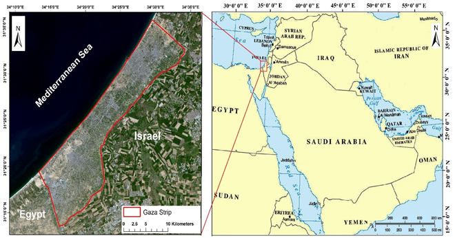
Figure-1. Study Area: Gaza Strip

2.2. Materials

2.2.1. TM and ETM+

Landsat satellite has been providing with the largest perpetual measurements of satellite-based remotely sensed observational data. It provides the satellite data with medium level spatial resolution and is helpful to monitor the global change. Table 1 shows the characteristics of TM and ETM7+ [25]. The data for TM and ETM+ is acquired from USGS Website obtained by specific path and row. Gaza Strip is covered by two paths and two rows namely, path/row 174/38 and path /row 175/38 (Figure 2).

Table-1. Specific characteristics of TM5 and ETM 7

ETM+ Bands	TM Bands	Name	Wavelength	Resolution
ETM+ 1	TM 1	Blue	0.45 - 0.52 µm	30 m
ETM+ 2	TM 2	Green	0.52 – 0.60 µm	30 m
ETM+ 3	TM 3	Red	0.63 – 0.69 µm	30 m
ETM+ 4	TM 4	NIR	0.76 – 0.90 µm	30 m
ETM+ 5	TM 5	MIR1	1.55 – 1.75 µm	30 m
ETM+ 6	TM 6	Thermal	10.4 – 12.50 µm	30 m
ETM+ 7	TM 7	MIR2	2.08 – 2.35 µm	30 m
ETM+ 8	-	Panchromatic	0.551 - 0.981 µm	15 m

Source: reference [25]

2.2.2. Ground-Based Observation Data

Ground measurements of PM10 concentration inside Gaza Strip are not available. However, PM10 concentration data is collected from ten air quality monitoring stations around the study area (Figure 2). PM10 concentration measurements are obtained using an automated instrument. The instrument automatically records PM10 concentration every 5 minutes. The data is then processed by special computer monitoring systems in the ground stations. This monitoring instrument has passed rigorous testing to be a precise Instrument and is harmless for humans and environment [26]. Moreover, an algorithm to estimate PM10 concentration has been developed based on 15 years data of Landsat images and PM10 ground measurements.

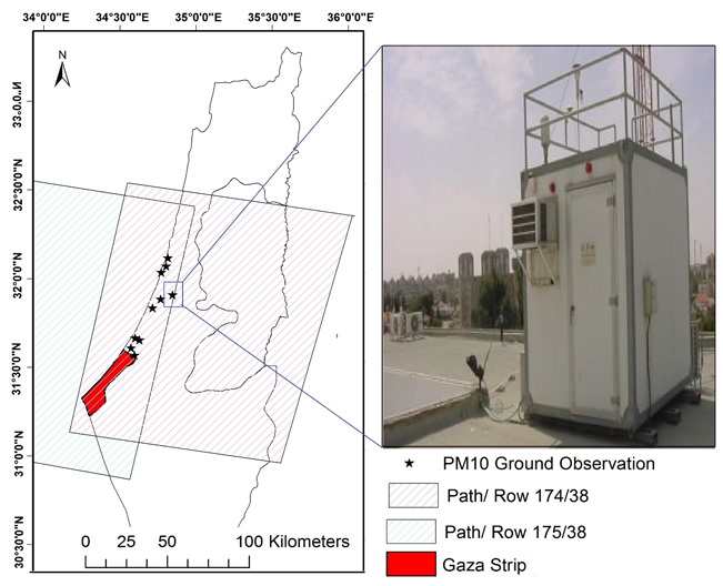
Figure-2. Path/Row of TM and ETM+ and Ground Observation location

2.3. Method

2.3.1. Geometric Correction

Geometric distortion is a commonly found error in raw multispectral satellite images, primarily because of the displacement in satellite position. These errors are to be removed before the manipulation of such images. Geometric distortion in an image is resolved by using resampling technique, taking minimum five ground control points (GCPs) on a base map and comparing it with satellite images of the study area. On May 31^st 2003, one of the sensors of ETM+ failed to scan called the Scan Line Corrector (SLC), which lost an approximate of 22 percent data. To fill the gap between scan lines, an algorithm has been used which is developed by Scaramuzza and Micijevic [27].

2.3.2. Radiometric calibration

Almost every satellite image contains cloud fraction and cloud shadow in it which causes the surface reflection to be reduced or lost completely. It is important to apply cloud masking. One of the Cloud and cloud shadow detection methods for Landsat is called Fmask, an algorithm developed by Zhu and Woodcock [28] for Landsat imagery. It gave an accuracy of about 94.6%. This method has been used in different researches [29, 30] and presented highly accurate results. We applied Fmask on our satellite data, for the detection and masking of cloud and cloud shadow. Satellite data manipulation requires pre-processing of the images, most important of which is radiometric calibration.

The basic goal of radiometric calibration in this research, is to extract the atmospheric reflectance of visible bands. Radiometric correction is performed by converting the value of Digital Number (DN) into radiance as equation (1), given by Chander, et al. [31].

(1)

Where, L is radiance at sensor expressed in Wm^-2 Sr^-1 µm^-1, λ is band number, Bias is band specific multiplicative rescaling factor from Metadata of TM and ETM+, Gain is band specific additive rescaling factor from Metadata of TM and ETM+ and DN is digital number.

Converting spectral radiance to top of atmosphere reflectance (TOA), for combined atmospheric reflectance and surface reflectance, is calculated with the following equation (2), [3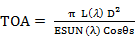2]

(2)

Where, TOA is the top of atmospheric reflectance at sensor, D is earth-sun distance in astronomical units [31] ESUN is mean solar exo-atmospheric irradiances (W/m²/sr/µm) [31] and θs = solar zenith angle (degree) (Metadata of TM and ETM+).

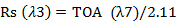
It is important to retrieve the surface reflectance prior to calculating the atmospheric reflectance for remote sensing data. For the respective study, surface reflectance is calculated by manipulating the relationship between three visible bands (blue, green and red) and the Mid Infrared (MIR) band at 2.1 µm. It is assumed that atmospheric haze does not significantly affect MIR band data, or else it can be retrieved from MIR band because to some extent, surface reflectance is correlated across different bands to each other. A number of studies showed accurate results by measuring surface reflectance of visible bands from MIR [33]. For this research, surface reflectance of the visible bands are calculated using equation (3, 4 and 5), given by Lim, et al. [18].

(3)

(4)

(5)

Where, Rs is the surface reflectance of visible bands, blue green and red. TOA (λ7) is the total reflectance at sensor of MIR band.

TOA is the sum of atmospheric reflectance and surface reflectance. The atmospheric reflectance is extracted using a simple form of the equation (6). This equation is also used by Popp, et al. [33]

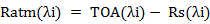(6)

Where, Ratm is the atmospheric reflectance (i=1, 2, 3... Corresponding to wavelength for satellite).

2.3.3. PM10 Algorithm Model

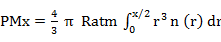
Mie Aerosols Scattering Theory has been applied to estimate the spectral optical depth and aerosol phase function. It is based on the imaginary index and aerosol size distribution [34, 35].

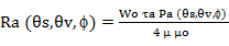(7)

On the other hand, atmospheric reflectance caused by Molecule Rayleigh scattering, is found by Liu, et al. [36]

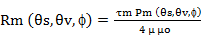(8)

Where, Ra is the atmospheric reflectance caused by Mie Aerosols scattering, Rm is the atmospheric reflectance caused by molecule Rayleigh scattering, θs is the solar zenith angle, θv is the viewing zenith angle, φ is the relative azimuth angle, Wo is the single scattering albedo, τa is aerosol optical thickness caused by aerosols, τm is the aerosol optical thickness caused by molecules, Pa is the aerosol scattering phase function, Pm is the rayleigh scattering phase function, µ is the cosines of the view directions and µο is the cosines of the solar directions.

The atmospheric reflectance is the sum of Ra and Rm [37].

Ratm = + (9)

The method can be applied to satellite imagery. i.e. For TM or ETM+ band 1. So, τa has been arranged by Xia [38] in equation (10)

τa = Ratm (10)

By ignoring Rm [39, 40] Equation (10) can be modified as Equation (11).

τa = Ratm (11)

Where, τa is the AOT. Parameters such as µ, µο, Wo, Pa, θs, θv and φ can be easily estimated by separate equations to presents as a coefficient value (A₀). Equation (11) can be written as Equation (12).

AOT = (A₀) Ratm (12)

Equation (8) is re-written for selected bands of TM and ETM+ as Equation (9).

AOT (λ) = A₀ Ratm (λ₁) + A₁ Ratm (λ₂) + A₂ Ratm (λ₃) (13)

Where, Ratm is the atmospheric reflectance (i=1, 2, 3... Corresponding to wavelength for satellite), Aj is the algorithm coefficient (j=0, 1, 2), it is determined empirically. The relation between PM and AOT is obtained for a single homogeneous layer of atmosphere which contain spherical aerosol particulates. The mass concentration at the surface is obtained after drying the sampled air, given by Koelemeijer, et al. [41].

(14)

Consequently, it is concluded that against AOT, the parameter of PM exhibits a better correlation directly. By utilizing the information resulting from spectral AOT analysis, PM10 concentration has been extracted. Several studies suggest that AOT and PM10 have a strong linear correlation where, R is more than 0.8 [42, 43]. Gupta, et al. [44]; Slater, et al. [45] and Engel-Cox, et al. [46] also analyzed the correlation between PM concentrations and AOT measurements by linear equation. By taking AOT as a substitute in terms of PM10 equation (13), PM10 algorithm with spectral reflectance of multi-band wavelengths (λi) is simplified as Equation (15).

PM10 = A₀ Ratm (λ₁) + A₁ Ratm (λ₂) + A₂ Ratm (λ₃) (15)

Table 2 shows a number of studies suggest that PM10 and atmospheric reflectance show linear correlation between them. Where, R was more than 0.8.

Table-2. Several Previous PM10 Regression Based on Landsat images

Name	Equation	correlation coefficient
Lim, et al. [17]	A0 R1 + A1 R3	R= 0.83
Nadzri, et al. [16]	369 R1 + 253 R2- 194 R3	R=0.888
Lim, et al. [18]	A0+A1 R1 +A2 R2+A3 R3	R= 0.908
Saleh and Hasan [47]	472 R1 – 419 R2 +307 R3	R= 0.833

2.3.4. Classification and Accuracy Assessment

Image classification methods are divided into two broad categories i.e. supervised and unsupervised. Each of the approaches has its own advantages as well as disadvantages; however, it is more likely to get maximum accuracy by supervised image classification technique than by unsupervised method [48, 49]. So, to carry out this study, both images of Landsat have been classified into thematic maps by performing supervised classification using maximum likelihood technique. Two major classes are identified which are urban area and non-urban area. Accuracy assessment is calculated by using ground data. Error matrices are then generated to analyze the user’s accuracy, producer’s accuracy and over all classification accuracy.

3. RESULTS AND DISCUSSION

3.1 Atmospheric Reflectance Extraction and Validation

Atmospheric reflectance of visible bands were extracted using equation (6), which needs to be validated. Ground measurement of surface reflectance or atmospheric reflectance on varying wavelengths are unavailable. However, Dark Object Subtraction Method (DOS) has been practiced to validate the atmospheric reflectance of visible band. Shadow area is a crucial component of this method, it employs the assumption that solar irradiance did not reach ground surface, instead reflectance from atmosphere gets recorded due to interaction between irradiance and atmospheric pollutants.

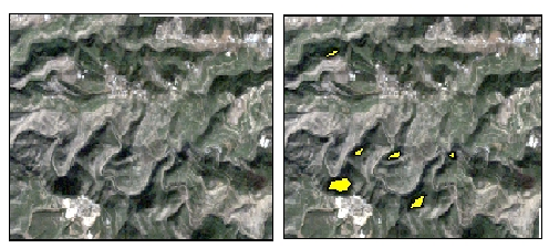
Figure-3. Dark Area (Shadow) by yellow boundary

Figure 3 shows the shadow area, represented by yellow color, is extracted to present TOA of visible band. Hence, to validate the atmospheric reflectance of visible bands, 16 images of Landsat for different seasons and years have been used. Atmospheric reflectance of all three visible bands strongly correlates with TOA of the corresponding bands over the shadow area where, correlation coefficient (R) > 0.95, Root Mean Square Error (RMSE) is nearly zero and P = 0 (Figure 4).

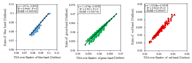
Figure-4. Validation of Atmospheric Reflectance of three Visible Bands

3.2. Estimating PM10 Model and Validation

This research approach analyzes the temporal vibration of PM10 concentration during the years 2000-2014 over Gaza Strip. Therefore, 11 years of ground data and satellite images have been utilized to create the PM10 algorithm and four years (2002, 2006, 2010 and 2014) have been used for the validation of this algorithm. The atmospheric reflectance for blue, green and red bands were determined using equation (6), as shows in figure 5. For the study, atmospheric reflectance values are averaged using the kernel size (7x7), which is adjusted at the ground measurements of 45 minutes before the passing of satellite above the study area due to lowest RMSE and highest R.

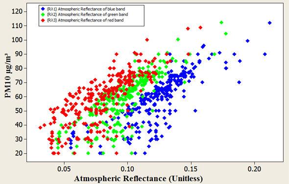
Figure-5. Atmospheric Reflectance of Three Visible Bands against PM10 measurement

A linear regression is used to create PM10 algorithm using Minitab software (Minitab 16.2.1), based on the lowest value of RMSE, a highest R and lowest (P). Where the R= 0.86, RMSE = 9.71 µg/m³ and P = 0. The PM10 algorithm is as below equation (16).

(16)

Where, PM10 is the PM10 concentration (µg/m³), Ratm (λ₁), Ratm (λ₂) and Ratm (λ₃) are the atmospheric reflectance of visible bands, blue, green and red respectively.

In addition, Figure 6 shows statistical results of regression such as probability plot, versus order, versus fits and histogram.

The results of validation by four years data average (2002, 2006, 2010 and 2014) show that the developed multispectral algorithm worked perfectly for this study. It gives average accuracy where, R = 0.88, RMSE = 10.83 µg/m³ and P = 0. (Figure 7A). Furthermore, the lowest validation is recorded on 12/2/2006 where, R = 0.811, RMSE = 7.15 µg/m³ and P < 0.003 (Figure 7 B). While, the highest validation is observed on 20/6/2014 where, R = 0.929, RMSE = 8.92 µg/m³ and P = 0. (Figure 7 C).

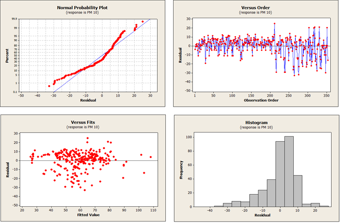
Figure-6. Statistical Result of the PM10 Regression

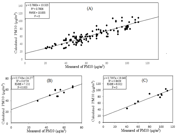
Figure-7. Validation results of the regression. (A) The average validation of four years; (B) The lowest validation on 12/2/2006 and (C) The highest validation on 20/6/2014

3.3. Temporal Variations of PM10 Concentration and Urbanization Extent

Table 3 shows the Images of TM and ETM+ that are used to establish the annual temporal variation of PM10 concentration over study area during the period 2000-2014.

Seasonal mean of PM10 concentration is obtained during the season time, ex: spring of 2000 is from 21 of March to 21 of June. We obtained the yearly mean by averaging the four seasons of the year.

Table-3. Years and months of image acquisition of TM and ETM+ which have been used to analyze PM10 over Gaza Strip.

Year

Jan

Feb

Mar

Apr

May

Jun

Jul

Aug

Sep

Oct

Nov

Dec

2000

x

xx

x

x xx

xxx

x

xx

x

2001

x

xx

x

xx

x

x

x

2002

xx

x

x

x

x

xx

2003

x

x

x

x

xx

x

x

x

x

2004

x

xx

xx

xx

x

xx

xx

x

2005

x

x

xx

xx

x

xx

xx

x

x

x

x

2006

x

x

x

xx

x

xx

x

x

x

x

2007

xx

x

x

x

xxx

x xx

xx

x

x

xx

xx

2008

x

x

x

xx

x

x

x

2009

x

x

x

xx

x

xx

xx

x

xx

xx

2010

x

x

x

xx

x

x

xx

xxx

2011

xx

x

x

xx

x

xx

xx

x

x

2012

x

x

xxx

x

xx

xx

xx

xxx

xx

x

2013

xx

x

xx

xx

xxx

xx

x

x

x

2014

xx

x

x

xx

x

xx

xx

x

x

Note: x, xx and xxx indicates availability of the image(s) of Landsat in the corresponding months

The general trend spread over 15 years (2000-2014) is shown in figure 8, where the maximum, minimum and the mean annual PM10 concentration have a positive trend line which leads to establish the premise that PM10 concentration has increased during these years over Gaza Strip.

Figure 8 shows the average yearly concentration for PM10. During the year 2000, the maximum, minimum and average recorded PM10 concentrations are 102 µg/m³, 28 µg/m³ and 65 µg/m³ respectively. It increases to a maximum of 120 µg/m³ a minimum of 33 µg/m³ and an average of 71 µg/m³ during 2000-2002. The year 2003 shows decrease in minimum (31 µg/m³) and mean (68.5 µg/m³) PM10 concentrations while, it shows increase in minimum (124 µg/m³) concentration. From 2004 to 2006, the maximum and mean PM10 concentrations decrease to 119 µg/m³ and 71 µg/m³ respectively but the minimum concentration shows an increase of about 38 µg/m³. During the years 2007-2009, decrease in minimum, and mean concentration is shown which reaches to be 36 µg/m³ of minimum and 75.8 µg/m³ of mean concentration while an increase of 135 µg/m³ is shown in maximum concentration. The results for 2010 show that PM10 concentration for maximum, minimum and average concentration decreased and reached to a maximum of about 134 µg/m³, the average of 71.5 µg/m³ and a minimum of about 32 µg/m³. During the years 2011–2014, there is an increase in the minimum, maximum and mean concentration of PM10 which reached the highest concentration overall during the 15 years, where the min is 45 µg/m³, the max is 144 µg/m³ and mean concentration is recorded to be 85.1 µg/m³. Pattern variation of annual mean PM10 concentration is clearly shown in figure 9

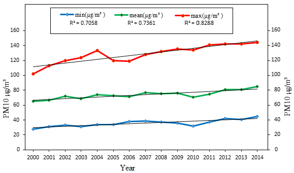
Figure-8. Trend Line variation of annual minimum, mean and maximum PM10 concentration over Gaza Strip during the years 2000-2014

Landsat TM image of 2000 and ETM+ of 2014 have been classified based on Maximum Likelihood technique, categorized into two classes i.e. urban area and non-urban area (fig. 10). Classification result (Table 4) represents urban area to be 79 Km² in 2000, which is 21.64 % of total area while non-urban area is calculated to be 286 Km² which is 78.36 % of the total area. Results reveal that in 2014 (Table 4), urban area increased up to 169 Km² (46.3 %). This shows an extremely high urban growth rate from 2000 to 2014. The overall accuracy of the maps derived from TM and ETM+ stood as 93% and 91% for 2000 and 2014 respectively.

Table-4. LULC results of the Gaza Strip during the years 2000 and 2014

Classes	. 2000 . Area (Km2) Area (% Age)	2014 . Area (Km2) Area (% Age)
Urban Area	79 21.64	169 46.3
Non-Urban Area	286 78.36	196 53.7

The PM10 concentrations show an overall increase during the years 2000-2014. To relate this increase with urbanization and accelerated rate of anthropogenic activities. Classification result shows that urban area over Gaza Strip especially Gaza City, has experienced increase during the years 2001-2014. This is evident from the Figure 10, where the area around Gaza City shows noticeable increased urban extent. The population of Gaza Strip has also increased to be 1.95 million in 2014 while, it was 1.1 million in the year 2000. This population growth led to an increase in the number of motor vehicles across Gaza Strip, which is estimated to be about 80,000. So, we can conclude that PM10 concentration over urban area shows increasing trend due to expansion of the urban area and industrialization. Urbanization and population growth have strongly affected PM10 level and boosted its concentration in the atmosphere during 2000-2014 over the Gaza Strip.

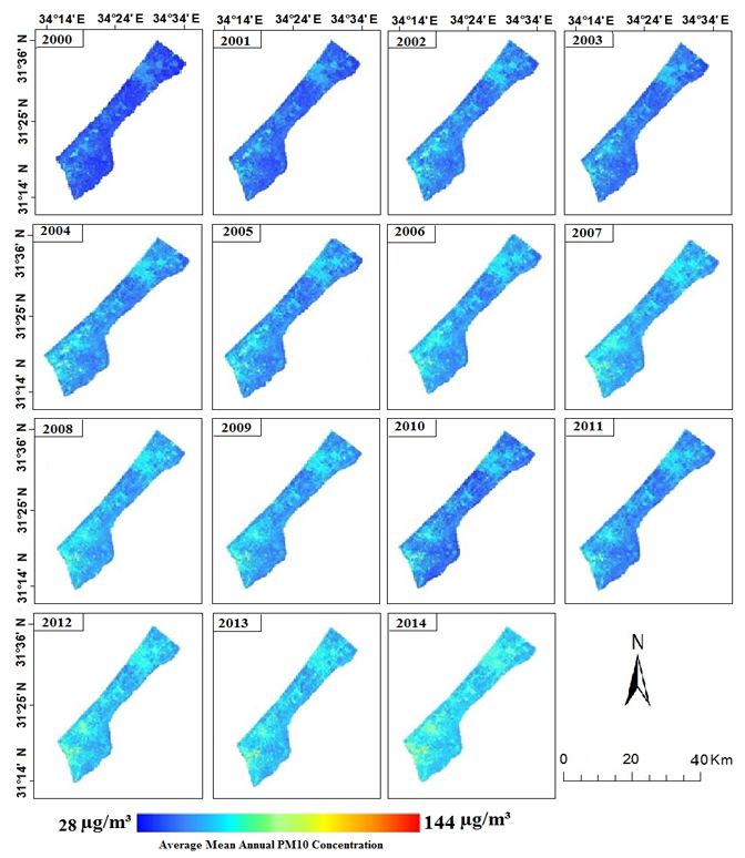
Figure-9. Pattern variation of annual mean PM10 concentration over Gaza Strip during the years 2000-2014

The effects of siege in the area leave strong imprints on the environment. It results in the usage of electricity generators by a large population, to compensate the power shortage experienced due to country’s inability to run its power generation plants. This is due to the fuel shortage for these plants. According to an estimation, about 100,000 generators per day are being used that consume almost 500,000 liters oil every day.

Another factor influencing the PM concentration in atmosphere is precipitation. It causes reduction in the amount of pollutant particles and gaseous molecules suspended in the air, during a rainfall season [50]. Rainfall is an active agent to wash away the large amount of tiny particles from the atmosphere. In case of no/less rainfall, the air remains loaded with particulate matter. Therefore, annually averaged data for rainfall from Ministry of Agriculture (MoA) [51] is analyzed for the respective time period (Figure 11). Statistics show a sharp decrease in rainfall quantity during the years, which is a potential cause of high PM10 concentration in study area

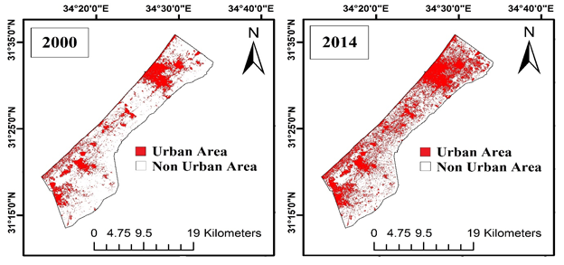
Figure-10. Classified Map for the years 2000 and 2014

.

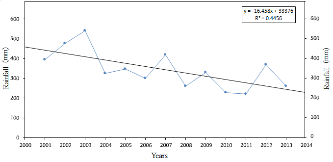
Figure-11. Average Annual Rainfall over Gaza Strip.

Source: Acquired from Palestinian Ministry of Agriculture (MoA).

4. CONCLUSION

• The atmospheric reflectance for Landsat visible bands has been validated using (DOS) method, using the assumption that solar irradiance did not reach ground surface, instead reflectance from atmosphere gets recorded due to interaction between irradiance and atmospheric pollutants.

• Atmospheric reflectance of the visible bands strongly correlates with TOA of the corresponding bands over the shadow area.

• We developed an algorithm to estimate the PM10 concentration over Gaza Strip based on Landsat image data and ground monitoring stations data for eleven years while, four years data has been used to validate the algorithm. The precision suggests that we can monitor PM10 concentration on small area or regional scale using Landsat observations.

• Analysis results give a positive trend line of PM10 concentration which shows an average increase in its concentration during the years 2000-2014 over the area.

• Urbanization and population have strongly affected the PM10 concentration where the highest concentration is found to be over urban area of Gaza Strip and is constantly increasing. Other factors include constantly decreasing rainfall which promoted PM10 accumulation.

5. RECOMMENDATIONS

It is recommended that Government of Palestine and WHO encourage the policy making and law implementation to control the air pollution in Gaza Strip and eradicate its sources and key factors, as this has become a rapidly growing problem presently which is affecting the health of a large portion of population as well as environment in the area. If the pollutants emission increases with the same pace it would become an uncontrollable hazard in the coming decades.

Funding: This study received no specific financial support.

Competing Interests: The authors declare that they have no competing interests.

Contributors/Acknowledgement: We thank COMSATS Institute of Information Technology and Department of Meteorology for providing the opportunity to carry out this research. We also thank Dr. Aqeel Ahmed Kidwai for the guidance, and our colleagues for the support and insights that greatly assisted the research.

REFERENCES

[1] H. Mayer, "Air pollution in cities," Atmospheric Environment, vol. 33, pp. 4029-4037, 1999. View at Google Scholar 

[2] R. Williams, J. Suggs, A. Rea, K. Leovic, A. Vette, C. Croghan, L. Sheldon, C. Rodes, J. Thomburg, A. Ejire, M. Herbst, and W. Sanders, "The research triangle park particulate matter panel study: PM mass concentration relationships," Atmospheric Environment, vol. 37, pp. 5349– 5363, 2003. View at Google Scholar | View at Publisher

[3] I. Adamson, H. Prieditis, and R. Vincent, "Pulmonary toxicity of an atmospheric particulate sample is due to the soluble fraction," 1999.

[4] J. H. Seinfeld and S. N. Pandis, Atmospheric chemistry and physics from air pollution to climate change. London: Wiley, 1998.

[5] M. I. Shahzad, N. E. Janet, W. Jun, C. R. James, and C. W. Pak, "Estimating surface visbility at Hong Kong from ground- based LIDAR, sun photometer and operrational MODIS product," Journal of the Air &Waste Mangment Associate, vol. 63, pp. 1098-1110, 2013. View at Google Scholar | View at Publisher

[6] J. Haywood and O. Boucher, "Estimates of the direct and indirect radiative forcing due to tropospheric aerosols: A review," Reviews of Geophysics, vol. 38, pp. 513–543, 2000. View at Google Scholar | View at Publisher

[7] WHO, "Air quality guidelines global update 2005," Report on a Working Group meeting, 18–20 October, Bonn2005.

[8] M. Kampa and E. Castanas, "Human health effects of air pollution," Environmental Pollution, vol. 151, pp. 362-367, 2008. View at Google Scholar 

[9] National Ambient Air Quality Objectives for Particulate Matter, "Science assessment document," Palestinian Central Bureau of Statistics (PCBS, 2014), 1998.

[10] N. Soulakellis, N. Sifakis, M. Tombrou, D. Sarigiannis, and K. Schäfer, "Estimation and mapping of aerosol optical thickness over the city of Brescia - Italy using diachronic and multiangle SPOT 1, 2 & 4 imagery," Geocarto International Journal, vol. 19, pp. 57-65, 2004. View at Google Scholar | View at Publisher

[11] J. Amanollahi, C. Tzanis, A. M. Abdullah, M. F. Ramli, and S. Pirasteh, "Development of the models to estimate particulate matter from thermal infrared band of landsat enhanced thematic mapper," International Journal of Environmental Science and Technology, vol. 10, pp. 1245-1254, 2013. View at Google Scholar | View at Publisher

[12] C. Q. Lin, Y. Li, Z. B. Yuan, K. H. Alexis, X. J. Deng, T. K. L. Tse, J. C. H. Fung, C. C. Li, Z. Y. Li, and X. C. Lu, "Estimation of long-term population exposur to PM2.5 for dense urban areas using 1-km MODIS data," Remote Sensing of Environment, vol. 179, pp. 13–22, 2016. View at Google Scholar | View at Publisher

[13] K. WijeratneI and W. Bijker, "Mapping dispersion of urban pollution with remote sensing," International Archives of Photogrammetry, Remote Sensing, and Spatial Information Sciences, vol. 34, pp. 125-130, 2006. View at Google Scholar 

[14] S. Saleh, "Air quality over Baghdad City using earth observation and landsat thermal data," Journal of Chemical Information and Modeling, vol. 53, pp. 1689–1699, 2011. View at Google Scholar 

[15] O. Nadzri, Z. M. J. Mohd, H. S. Lim, and K. Abdullah, "Satellite retrieval optical thickness over estimating Arid Region: Case study over Makkah, Mina and Arafah, Saudi Arabia," Journal of Applied Sciences, vol. 10, pp. 3021-3031, 2010. View at Google Scholar | View at Publisher

[16] O. Nadzri, M. Z. Matjafri, and H. S. Lim, "Estimating particulate matter concentration over Arid Region using satellite remote sensing: A case Study in Makkah, Saudi Arabia," Modern Applied Science, vol. 4, pp. 131–142, 2010. View at Google Scholar | View at Publisher

[17] H. S. Lim, M. Z. Matjafri, and K. Abdullah, "Algorithm for air quality mapping using satellite images," pp. 383-308, 2010.

[18] H. S. Lim, M. Z. MatJafri, K. Abdullah, N. M. Saleh, and A. Sultan, Remote sensing of PM10 from LANDSAT TM imagery. Thailand: Acrs Chiang Mai, 2004.

[19] A. Ung, L. Wald, T. Ranchi, C. Weber, and J. Hirsch, "Air pollution mapping: Relationship between satellite made observation and air quality parameters," presented at the 12th International Symposium. Transport and Air Pollution, Avignon, France, 2003.

[20] A. Ung, C. Weber, G. Perron, J. Hirsch, and J. Kleinpeter, "Air pollution mapping over a city – virtual stations and morphological indicators," presented at the 10th International Symposium “Transport and Air Pollution”, Colorado, USA, 2001.

[21] A. Ung, L. Wald, T. Ranchin, C. Weber, J. Hirsch, G. Perron, and J. Kleinpeter, "Air pollution mapping: A new approach based on remote sensing and geographical databases," Application to the city of Strasbourg. Photo-Interpretation, pp. 3-4, 2000.

[22] A. Retalis, C. Cartalis, and E. Athanassious, "Assessment of the distribution of aerosols in the area of Athens with the use of landsat thematic mapper data," International Journal of Remote Sensing, vol. 20, pp. 939-945, 1999. View at Google Scholar | View at Publisher

[23] L. Wald and J. M. Baleynaud, "Observed air quality over city of Nantes by means of landsat thermal infrared data," International Journal of Remote Sensing, vol. 20, pp. 947-959, 1999. View at Google Scholar | View at Publisher

[24] Palestinian Central Bureau of Statistics (PCBS), 2014.

[25] NASA, "Landsat 7 science data user handbook. Retrieved from http://Landsathandbook.gsfc.nasa.gov/handbook.html. [ Accessed 15 May 2010]," 2010.

[26] National Air Quality Monitoring Network of the Ministry of Environment of Israel (NAQM), 2010.

[27] P. Scaramuzza and E. Micijevic, "SLC gap-filled products phase one methodology preliminary assessment of the value of landsat 7 ETM+ data following scan line corrector malfunction." Retrieved from http://landsat.usgs.gov/documents/SLC_Gap_Fill_Methodology.pdfUSGS&NASA . [Accessed June 2003], 2004.

[28] Z. Zhu and C. E. Woodcock, "Object-based cloud and cloud shadow detection in landsat imagery," Remote Sensing of Environment, vol. 118, pp. 83-94, 2012. View at Google Scholar | View at Publisher

[29] Y. Liu, S. Wei, and D. Xiangzheng, "Changes in crop type distribution in Zhangye City of the Heihe River Basin, China," Applied Geography, vol. 76, pp. 22-36, 2016. View at Google Scholar | View at Publisher

[30] X. Quana, H. Binbin, Y. Marta, Y. Changming, L. Zhanmang, Z. Xueting, and L. Xing, "A radiative transfer model-based method for the estimation of grassland aboveground biomass," International Journal of Applied Earth Observation and Geoinformation, vol. 54, pp. 159–168, 2016. View at Google Scholar | View at Publisher

[31] G. Chander, B. L. Markham, and D. L. Helder, "Summary of current radiometric calibration coefficients for landsat MSS, TM, ETM+, and EO-1 ALI sensors," Remote Sensing of Environment, vol. 113, pp. 893–903, 2009. View at Google Scholar | View at Publisher

[32] P. M. Mather, Computer processing of remotely-sensed images an introduction, 3rd ed.: John Wiley and Sons, 2004.

[33] C. Popp, D. Schläpfer, S. Bojinski, M. Schaepman, and K. I. Itten, "Evaluation of aerosol mapping methods using AVIRIS imagery. R. Green (Editor)," presented at the 13th Annual JPL Airborne Earth Science Workshop. JPL Publications, March 2004, Pasadena, CA, 10, 2004.

[34] M. D. King, Y. J. Kaufman, D. Tanre, and T. Nakajima, "Remote sensing of tropospheric aerosols from space: Past, present, and future," Bulletin of the American Meteorological Society, vol. 80, pp. 2229-2259, 1999. View at Google Scholar | View at Publisher

[35] H. Fukushima, M. Toratani, S. Yamamiya, and Y. Mitomi, "Atmospheric correction algorithm for ADEOS/OCTS acean color data: Performance comparison based on ship and buoy measurements," Advances in Space Research, vol. 25, pp. 1015-1024, 2000. View at Google Scholar | View at Publisher

[36] C. H. Liu, A. J. Chen, and G. R. Liu, "An image-based retrieval algorithm of aerosol characteristics and surface reflectance for satellite images," International Journal of Remote Sensing, vol. 17, pp. 3477-3500, 1996.

[37] E. Vermote, D. Tanre, J. L. Deuze, M. Herman, and J. J. Morcrette, "6S user guide version 2, second simulation of the satellite signal in the solar spectrum." Retrieved from http://www.geog.tamu.edu/klein/geog661/handouts/6s/6smanv2.0_P1.pdf, 1997.

[38] X. Xia, "Significant overestimation of global aerosol optical thickness by MODIS over land," Chinese Science Bulletin, vol. 51, pp. 2905-2912, 2006. View at Google Scholar | View at Publisher

[39] D. K. Paronis and J. N. Hatzopoulos, "Aerosol optical thickness and scattering phase function retrieval from solar radiances recorded over water: A revised approach," International Geoscience and Remote Sensing Symposium, vol. 4, pp. 1920-1922, 1997. View at Google Scholar 

[40] Y. J. Kaufman and D. Tanre, "Algorithm for remote sensing of tropospheric aerosol from Modis, Product ID: MOD04," 1998.

[41] R. B. A. Koelemeijer, C. D. Homan, and J. Matthijsen, "Comparison of spatial and temporal variations of aerosol optical thickness and particulate matter over Europe," Atmospheric Environment, vol. 40, pp. 5304-5315, 2006. View at Google Scholar | View at Publisher

[42] N. Sifakis, N. Soulakellis, D. Paronis, and R. Mavrantza, "Manual of EO image processing codes," Revised Reference Manual V.1.1, 2002.

[43] D. A. Chu, Y. J. Kaufman, G. Zibordi, J. D. Chern, M. Jietai, and L. Chengcai, "Global monitoring of air pollution over land from the earth observing system-terra moderate resolution imaging spectroradiometer (MODIS)," Journal of Geophysical Research, vol. 108, pp. 4661-4678, 2003. View at Google Scholar 

[44] P. Gupta, S. A. Christopher, and J. Wang, "Satellite remote sensing of PM and air qualliy assessment over global cities," Atmospheric Environment, vol. 40, pp. 5880–5892, 2006. View at Google Scholar | View at Publisher

[45] J. F. Slater, J. E. Dibb, J. W. Campbell, and T. S. Moore, "Physical and chemical properties of surface and column aerosols at a rural New England site during MODIS overpass," Remote Sensing of Environment, vol. 92, pp. 173–180, 2004. View at Google Scholar | View at Publisher

[46] J. A. Engel-Cox, C. H. Holloman, and B. W. Coutant, "Qualitative and quantitative evaluation of MODIS satellite censor data for regional and urban scale air quality," Atmospheric Environment, vol. 38, pp. 2495–2509, 2004. View at Google Scholar | View at Publisher

[47] S. A. H. Saleh and G. Hasan, "Estimation of PM10 concentration using ground measurements and landsat 8 OLI satellite image," Journal of Geophysics & Remote Sensing, vol. 3, pp. 1–6, 2014. View at Google Scholar 

[48] D. T. Peter and L. L. Michael, "Measuring praise and criticism: Inference of semantic orientation from association," ACM Transactions on Information Systems, vol. 21, pp. 315–346, 2003. View at Google Scholar 

[49] M. J. Butt, A. Waqas, M. F. Iqbal, G. Muhammad, and M. A. K. Lodhi, "Assessment of urban sprawl of Islamabad metropolitan area using multi-sensor and multi-temporal satellite data," Arabian Journal for Science and Engineering, vol. 37, pp. 101–114, 2012. View at Google Scholar | View at Publisher

[50] J. M. Yoo, Y. R. Lee, D. Kim, M. J. Jeong, W. R. Stockwell, P. K. Kundu, S. M. Oh, D. B. Shin, and S. J. Lee, "New indices for wet scavenging of air pollutants (O3, CO, NO2, SO2, and PM10) by summertime rain," Atmospheric Environment, vol. 82, pp. 226-23, 2014. View at Google Scholar | View at Publisher

[51] Ministry of Agriculture (MoA), "Rainfall report, general directorate of soil and irrigation, Palestine." Retrieved from http://www.apis.ps/documents/MoA_Final_rainfall_Report_2007-2008.pdf, 2008 & 2014.

Views and opinions expressed in this article are the views and opinions of the author(s), Journal of Asian Scientific Research shall not be responsible or answerable for any loss, damage or liability etc. caused in relation to/arising out of the use of the content.