


INVESTIGATING THE ROLE OF OIL PRICES IN THE CONVENTIONAL EKC MODEL: EVIDENCE FROM TURKEY

1Faculty of Economics & Administrative Sciences, University of Kyrenia, Kyrenia, Northern Cyprus, Via Mersin 10, Turkey
ABSTRACT
The present article tests the effect of oil price movements in the conventional Environmental Kuznet’s Curve of the Turkish economy. Contemporary time series analysis has been adapted with this respect. Results of the study reveal that oil prices and carbon emissions are in long-term equilibrium relationship in Turkey; carbon dioxide emissions converge to long-term paths as contributed by oil price changes very rapidly as much as 103.5 percent. The effects of oil prices on carbon dioxide emissions are negative and they are significant in proving that increases in oil prices lead to declines in the levels of carbon emissions. Finally, the major finding of this study confirmed the oil-induced EKC hypothesis in the case of Turkey.
© 2017 AESS Publications. All Rights Reserved.
Keywords : Oil , Environment, Kuznets’s Curve, EKC Multiple structural breaks, ECM, Turkey
Article History: Received: 3 December 2016, Revised: 4 January 2017, Accepted: 27 January 2017, Published: 22 February 2017
JEL Classification: C22, C51, Q50.
1. INTRODUCTION
The CO2 emissions from energy consumption have significantly increased in newly industrialized countries since the 1990s when compared to industrialized countries (Kasman and Duman, 2015). The deterioration of environmental quality has reached to alarming levels and raised concerns about global warming and climate change. Hence, understanding the reasons behind environmental degradation and its relation with economic growth has become increasingly important in recent years. The effects of economic growth on environment have become a common ground of research among economists (Kasman and Duman, 2015).
In 2004, oil accounted for 35% of the world energy demand. Fossil fuels as a group (coal, oil and natural gas) have accounted for 80% of the world energy demand. Rising oil price should encourage households and businesses to reduce consumption, purchase more products that are efficient and switch to renewable energy sources (Sadorsky, 2009). Therefore, oil markets are of major importance for the world’s economy (Al-Abdulhadi, 2014; Memis and Kapusuzoglu, 2015).
Some words are due for choosing the energy consumption. Energy consumption is one factor ‘whose direct and indirect environmental significance is indisputable’, the obvious reason is that interferences with nature also arise from the power that energy gives us to move and extract the matter. This is particularly relevant to nowadays since the material scale/throughput of rich economies is particularly high (Luzzati and Orsini, 2009).
Kasman and Duman (2015) suggest a long run cointegrated relationship among carbon emissions, energy consumption, real income, trade openness and urbanization for a panel of new EU member and candidate countries for the period 1992–2010. Heidari et al. (2015) show that there is a nonlinear relationship among CO2 emissions per capita, energy consumption per capita, and GDP per capita in five Asians countries. However, they indicated that economic growth in Singapore due to high level of per capita income leads to decrease in CO2 emission. Malaysia’s per capita income is located at the turning point, and expected that economic growth would lead to a reduction in CO2. In contrast, per capita income in Thailand, Indonesia and Philippines are slightly less than that turning point which is 4,686 USD and thus economic growth move together with CO2 emissions in these countries.
Alshehry and Belloumi (2015) investigate the dynamic causal relationships among energy consumption, energy price and economic activity in Saudi Arabia based on a demand side approach. The results indicate that there exists at least a long-run relationship between energy consumption, energy price, carbon dioxide emissions, and economic growth. Even though, the energy-led growth hypothesis is valid, the share of energy consumption in explaining economic growth is minimal. Energy price is the most important factor in explaining the economic growth. Hence, policies aimed at reducing energy consumption and controlling for CO2 emissions may not reduce significantly economic growth as also found in the case of Saudi Arabia by Alshehry and Belloumi (2015). Investing in the use of renewable energy sources like solar and wind power is an urgent necessity to control fossil fuel consumption and CO2 emissions.
Many studies have tested the validity of the environmental Kuznets curve (EKC) hypothesis which investigates the interactions between environmental pollution and gross domestic product (GDP) (Magnani, 2000; Luzzati and Orsini, 2009; Saboori et al., 2012; Kaika and Zervas, 2013; Shahbaz et al., 2013; Kapusuzoglu, 2014; Lau et al., 2014; Anatasia, 2015). Moreover, emerging countries due to the onset of accelerated growth path may not have paid much attention to the quality of the environment and nevertheless, after reaching a certain level of per capita income they demand for a healthy environment. Thus, an inverted U-shaped EKC might exist in countries and regions; turning points of their EKCs need to be investigated through empirical analysis (Heidari et al., 2015).
Some studies have investigated the relationship between carbon dioxide emissions and oil price (Henriques and Sadorsky, 2008; Sadorsky, 2009; Méjean and Hope, 2013). Majumdar and Parikh (1996) use oil prices and population to model the demand for the energy in India. Silk and Joust (1997) use oil prices to model the residential energy demand in the United States by looking at the investment climate for publicly traded alternative energy companies. Henriques and Sadorsky (2008) find that the stock prices of alternative energy companies respond more to a shock to technology stock prices (or a technology index) than they do to shocks to oil prices. Global warming issues have put CO2 emissions into the energy policy spot light. Any serious attempt to deal with global warming is going to reduce the dependancy on fossil fuels. Consequently, increases in carbon dioxide emissions, coupled with increased concern over global warming, are likely to lead to increase the consumption of renewable energy. However, Sadorsky (2009) presents that oil price increases have a smaller but negative impact on renewable energy consumption.
Al-Mulali et al. (2013) explored the relationship between urbanization, energy consumption, and CO2 emission in the MENA countries and found that there was a long run bi-directional positive relationship between urbanization, energy consumption, and CO2 emission. However, the significance of the long run relationship between urbanization, energy consumption, and CO2 emission varied across the countries based on their level of income and development.
Oil price have a statistically significant impact on energy consumption and energy consumption have impact on CO2 emissions and environment quality as documented in the literature. Therefore, oil price might have indirect effects on the levels of CO2 emission. Against this backdrop, the present article investigates the role of oil price in the conventional EKC in the case of Turkey. Turkey has been selected because it is one of the important developing countries, and is one of the huge poles of the energy industry. Sectoral developments are catalyst for energy consumption. For example, tourism growth leads to a growth in energy capacity and leads to increase in the level of pollution (Katircioglu, 2009). Oil price might influence economy wide patterns of resource use, and global environmental quality. In particular, the indirect and direct energy requirements of oil price are through to contribute significantly to the adverse environmental impacts from urbanization (Liu, 2009). Therefore, this study contributes to the existing literature by integrating oil prices into the conventional EKC framework in order to test the role of oil price movements for the changes in energy consumption and carbon emissions. To the best of our knowledge, the present study is the first of its kind as well as its modeling technique and country case are concerned in the relevant literature till the moment.
The rest of the article is structured as follows: Section 2 defines the theoretical setting of the present study; Section 3 introduces the data and methodology; Section 4 presents the empirical results and discussion, and section 5 concludes the study.
2. THEORETICAL SETTING
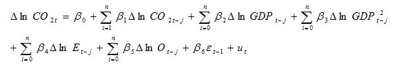
Environmental pollution is extensively peroxide by CO2 emissions (kt) as indicated in the relevant literature (Katircioglu, 2014). The starting point of the theoretical setting in this study is that oil price might be a determinant of CO2 emissions level through additional energy consumption and economic activity. In the conventional EKC framework, GDP is the main determinant of CO2 emissions. Because some countries might have an inverted U-shaped EKC, squared GDP (GDP2) is extensively used in the literature while some studies also consider the third power of GDP in the EKC framework. The energy economics literature suggest energy consumption as another important determinant of CO2 emissions, which is added to the relationship between CO2 emissions and (GDP) under the conventional EKC framework, in which an inverted U-shaped pattern of the EKC might still exist (Stern, 2004). In Turkey, it would be expected that oil price would lead to an increase in energy use and GDP and therefore, in pollution level. Therefore, the following oil price-induced EKC model is suggested in this study:
 (1)
(1)
Where CO2 refers to carbon dioxide emissions (kt), E signifies energy consumption (kt of oil equivalent), GDP is gross domestic product, and O stands for oil price proxy. The parameters of  and
and  and are the coefficients of regressors. The oil price-induced EKC model in equation (1) could be expressed in a double logarithmic regression equation to capture the growth impacts over the economic long-term period (Katircioglu, 2010):
 (2)
(2)
Where at period t, the terms “ln” stands for the natural logarithm of regressors in equation (2) while is the error disturbance.
The dependent variable in equation (2) might not immediately adjust to its long-term equilibrium path following any changes in its determinants. Therefore, the speed of adjustment between the short-run and the long-run levels of the dependent variable could be captured by estimating the following error correction model:
 (3)
(3)
Where  represents a change in CO2, E, GDP, GDP2 and oil price (O) while
 is the one period lagged error correction term (ECT), which is estimated from the residuals of equation (2). The ECT in equation (3) shows how quickly the disequilibrium between the short-term and long-term values of the dependent variable (CO2) is eliminated in each period. The expected sign of ECT would be negative (Gujarati, 2003).
3. DATA AND METHODOLOGY
3.1. Data
The data used in this research are annual figures covering the 1960–2010 period (World Bank, 2016) and the variables are (CO2) emission (kt), energy use (E) (kt of oil equivalent), constant GDP (2005 = 100), squared (constant) GDP (2005 = 100) (GDP2), and oil price (O) in Turkey.
3.2. Methodology
This study estimated the oil price-induced EKC model in Turkey. The second-generation econometric procedures that take multiple structural breaks into consideration is adapted in the study through Gauss codes. As a first step, the quasi (Generalized Least Squares (GLS)) based unit root tests, which were developed by Carrion-i-Silvestre et al. (2009) considering multiple structural breaks up to five are carried out for the time series in the study. This is due to the fact that series exhibit multiple breaks over the years as can also be obsereved in Figure 1. In the second step, cointegration tests (by Maki (2012)) which again considered multiple structural breaks untill five are carried out to confirm the existence of the cointegrating vector in equation (2). In the third step, long-run and short-run models plus ECT are estimated by using the Dynamic Ordinary Least Squares (DOLS) method. Finally, Granger causality tests through the block exogeneity approach, impulse response functions plus variance decompositions are also estimated to provide further support to the earlier results of this study. It is important to note that details of these appoaches are not provided here due to the fact that they are available and described in the econometric theory and related textbooks.
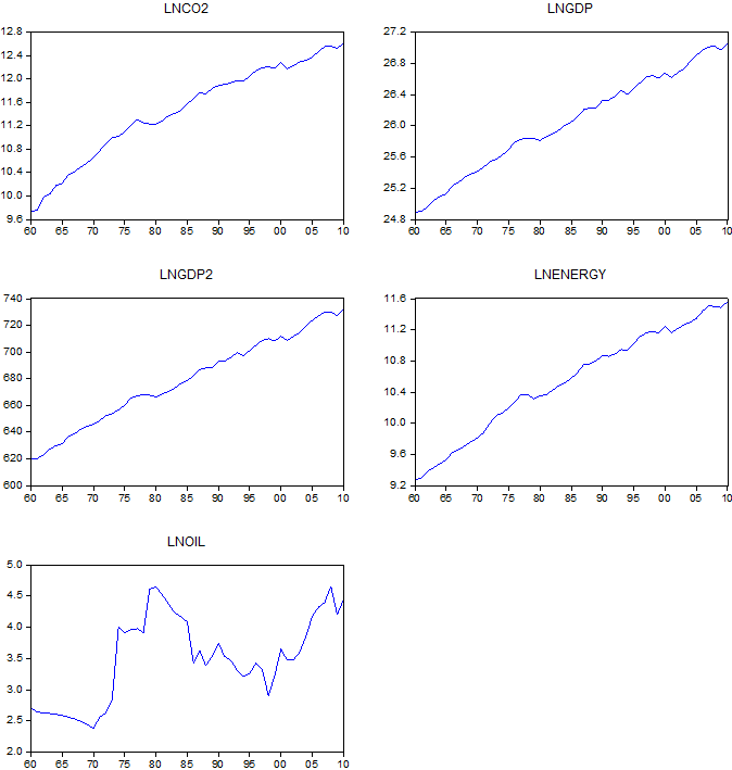
Figure-1. Time Series Plot of Variables under Consideration in the Natural Logarithm in Turkey
Source: Data have been gathered from World Bank (2016) and plotted by the author.
4. RESULTS AND DISCUSSION
4.1. Unit Root Test Results
Table 1 provides the GLS-based unit root test results from Carrion-i-Silvestre et al. (2009) for the variables under consideration. Unit root tests suggest three successful and significant structural break points in the series as can be seen from Table 1. By taking these break years into account, unit root tests reveal that all of the series under consideration are non-stationary at their levels; this is because the null hypothesis of a unit root cannot be rejected in the case of each variable. However, these series become stationary at their first differences since the null hypothesis of a unit root can be rejected again in the case of each variable. Results from GLS-based unit root tests suggest that lnCO2, lny, lnE, and lnO are integrated of order one, I (1), in the present study; therefore, it is likely that equation (1) of the present study might be a cointegration model.
Table-1. Unit root tests under multiple structural breaks
| Turkey | Levels | Year breaks | ||||
| PT | MPT | MZα | MSB | MZt | ||
| lnCO2 | 7.74 [5.54] |
7.79 [5.54] |
-22.20 [-30.48] |
0.15 [0.13] | -3.33 [-3.87] |
1977; 1980; 1987 |
| lny | 8.32 [5.54] |
8.50 5.54] |
-22.33 [-30.48] |
0.15 [0.13] | -3.18 [-3.87] |
1977; 1980; 1987 |
| Lny2 | 8.42 [5.54] |
8.59 [5.54] | -20.12 [-30.48] |
0.15 [0.13] | -3.17 [-3.87] |
1977; 1980; 1987 |
| lnE | 10.04 [5.80] |
9.65 [5.80] | -18.94 [-31.02] |
0.16 [0.12] | -3.07 [-3.91] |
1977; 1981; 1987 |
| lnO | 9.25 [5.98] |
9.52 [5.98] | -22.16 [-33.14] |
0.14 [0.12] |
-3.30 [-4.06] |
1970; 1979; 1998 |
| First differences | ||||||
| ΔlnCO2 | 3.83 [5.54] |
3.68 [5.54] | -24.72 [-17.32] |
0.14 [0.16] | -3.51 [-2.89] |
0.00 |
| Δlny | 3.89 [5.54] | 3.76 [5.54] |
-24.78 [-17.32] |
0.14 [0.16] | -3.50 [-2.89] |
0.00 |
| Δlny2 | 3.88 [5.54] |
3.77 [5.54] | -24.78 [-17.32] |
0.14 [0.16] |
-3.50 [-2.89] |
0.00 |
| ΔlnE | 3.89 [5.54] |
3.73 [5.54] | -24.77 [-17.32] |
0.14 [0.16] | -3.51 [-2.89] |
0.00 |
| ΔlnO | 3.56 [5.54] |
3.67 [5.54] | -24.96 [-17.32] |
0.14 [0.16] |
-3.52 [-2.89] |
0.00 |
Note: Year breaks are determined by using the unit root tests of Carrion-i-Silvestre et al. (2009). * denotes the rejection of the null hypothesis of a unit root at the customary 0.05 significance level. Numbers in square brackets are critical values from the bootstrap approach.
4.2. Cointegration Tests under Multiple Structural Breaks
All of the series in the present study are integrated of the same order; therefore, cointegration test for equation (1) employing Maki (2012) approach is suitable. Results of cointegration tests under multiple structural breaks are given in Table 2:
Table-2. Maki (2012) cointegration tests under multiple structural breaks
| Turkey | Completed Values [Critical Values] | Year breaks |
| Model 0 | -8.19 [-6.85, -6.30, -6.03]* | (1963; 1969; 1977; 1992; 2004) |
| Model 1 | -9.76 [-7.05, -6.49, -6.22]* | (1963; 1973; 1977; 1984; 2006) |
| Model 2 | -11.90 [-9.44, -8.86, -8.54]* | (1970; 1977; 1984; 1990; 2000) |
| Model 3 | - | - |
Note: The numbers in square brackets are critical values at the 0.05 significance level obtained from Table 1 of Maki (2012). * denotes rejection of the null hypothesis of ‘no cointegration’ at alpha 0.01 percent. The numbers in round brackets are structural breaks (year breaks) as determined by using Maki (2012) cointegration test.
It is seen that the null hypothesis of no cointegration can be rejected through the existence of various structural break years as can be seen in Table 2 and through two out of four models suggested by Maki (2012) as presented in the previous section of this study. Results from Maki (2012) reveal that equation (1) is a cointegration model and estimating the parameters in equation (2) would be robust in the long-term period. It is important to note that those break years which have been successfully obtained and provided in Table 2 are also added to estimate the long-term coefficients in equation (2) via dummy variables (Maki, 2012). Thus, Maki (2012) test suggests that carbon dioxide emissions in Turkey are in long term equilibrium relationship with its real income growth, energy consumption and oil price changes in Turkey.
Table-3. Long-run Estimates With the overall CO2 emissions
| Turkey | Constant | lnGDP | lnGDP2 | lnE | LnO | Trend |
| lnCO2 | -99.06* [-4.12] |
7.41* [4.08] |
-0.13* [-4.08] |
0.72* [4.92] |
-0.012*** [-1.73] |
-0.009** [-2.09] |
| K1 | K2 | K3 | K4 | K5 | R2 | DW |
-0.04 [-1.44] |
0.029 [1.12] |
-0.001 [1.14] |
-0.01 [-0.74] |
-0.03 [-1.17] |
0.99 | 1.98 |
Note: The numbers in square brackets are t ratios. Autocorrelation and heteroscedasticity problems in the model have been eliminated by means of the Newey-West approach. The five dummy variables in the models are: K1 (1963), K2 (1973), K3 (1977), K4 (1984) and K5 (2006) from Model 3 that includes a constant and a deterministic trend. *, **, and *** denotes statistical significance at the customary 0.01, 0.02, and 0.05 significance levels, respectively.
4.3. The Estimation of Long-Term Coefficients
Long-term coefficients as described in equation (2) are estimated through the DOLS approach and presented in Table 3. It is seen that the coefficient of GDP is positive and of squared GDP (GDP2) is negative and statistically significant. This finding is quite in parallelism with the inverted U-shaped EKC hypothesis. Energy consumption, on the other hand, exerts positive, statistically significant and inelastic effect on carbon emissions which indicates a damaging effect on the EKC as expected (β = 0.72, p < 0.01). Most importantly, the coefficient of oil price is elastic, negative and statistically significant (β = 0.012, p < 0.10), which suggests that one percent change in oil price would lead to 0.12 percent change in carbon emissions in the same direction which means “damages” on climate at further levels of oil price. This reveals that boosting oil price exerts negatively significant effects on climate changes in the case of Turkey that signals for unsuccessful energy policies. Finally, the results from Table (3) show that the coefficients of the break years are not statistically significant. The coefficient of intercept is negative and statistically significant which is quite reasonable denoting that without any change its determinants in equation (1) of this study carbon emission are likely to decline significantly.
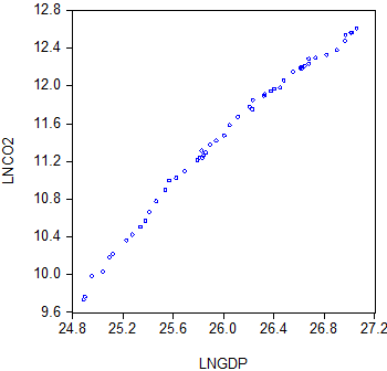
Panel-a. Conventional EKC
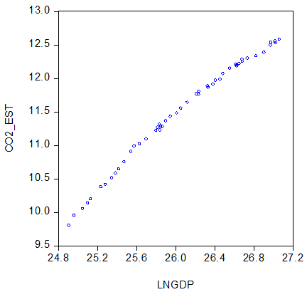
Panel-b. Revised EKC
Figure 2. Actual and Estimated EKCs for Turkey
Source: Graphs have been plotted by the author in EVIEWS software.
Before proceeding with the ECM regressions, it will be very helpful to provide the EKC figures in the case study with and without the oil price volume. Figure 2, which is based on the estimations from Table 3, plots the EKC for Turkey in two different EKC model options: (1) Conventional EKC without oil price but with estimated CO2 emissions with respect to GDP and energy consumption; (2) Revised EKC including oil price. Figure 2 shows that the EKC of Turkey is not an inverted U-shaped no matter oil prices are added or not. In other words, Figure 2 proves that in the existence or absence of oil prices the EKC of Turkey are in upward movements; thus, oil prices do not affect its shape in the longer periods.
Table-4. Conditional Error Correction Models Through The ARDL Approach and Short-term Coefficients
| Regressor | Coefficient | Standard Error | t-value | |
| ût-1 | -1.035 | 0.554 | -1.86 | |
| ΔlnCO2t-1 | 1.09 | 0.572 | 1.90 | |
| ΔlnCO2t-2 | 0.560 | 0.539 | 1.03 | |
| ΔlnCO2t-3 | 0.244 | 0.496 | 0.49 | |
| ΔlnCO2t-4 | 0.898 | 0.406 | 2.21 | |
| Δlnyt-1 | 15.698 | 13.558 | 1.15 | |
| Δlnyt-2 | -22.871 | 12.819 | -1.78 | |
| Δlnyt-3 | -12.334 | 11.340 | -1.08 | |
| Δlnyt-4 | -1.346 | 11.188 | -0.120 | |
| Δlny2t-1 | -0.310 | 0.253 | -1.22 | |
| Δlny2t-2 | 0.426 | 0.240 | 1.77 | |
| Δlny2t-3 | 0.233 | 0.215 | 1.08 | |
| Δlny2t-4 | 0.010 | 0.214 | 0.05 | |
| ΔlnEnergyt-1 | -0.412 | 0.545 | -0.75 | |
| ΔlnEnergyt-2 | -0.133 | 0.545 | -0.24 | |
| ΔlnEnergyt-3 | -0.230 | 0.520 | -0.44 | |
| ΔlnEnergyt-4 | -0.350 | 0.502 | -0.69 | |
| ΔlnOilt-1 | 0.001 | 0.034 | 0.05 | |
| ΔlnOilt-2 | 0.048 | 0.033 | 1.44 | |
| ΔlnOilt-3 | 0.019 | 0.034 | 0.58 | |
| ΔlnOilt-4 | -0.023 | 0.034 | -0.68 | |
| Intercept | 0.040 | 0.020 | 1.97 | |
Adj. R2= 0.141 S.E. of Regr. = 0.048, AIC = -2.928, SBC = -2.054, F-stat. = 1.353 |
Source: Results have been obtained by the author in EVIEWS software.
4.4. The Estimation of Error Correction Models
The ECM regression associated with cointegration model in equation (2) will be estimated as a next step. The results of ECM regression are provided in Table 4. The ECT term in equation (3), where lnCO2 is the dependent variable, is 0.898, statistically significant, and positive (β = 0.898, p < 0.10). This implies that lnCO2 (carbon dioxide emission) converge to its long-term equilibrium path by 89.8 percent speed of adjustment through the channels of energy consumption, real income, and oil price changes. The short-term coefficient of GDP (without squaring) is negative, elastic, and statistically significant at the second lag (β = -22.871, p < 0.10). Furthermore, the short-term coefficient of squared GDP (GDP2) is positive, inelastic, and statistically significant (β = 0.426, p < 0.10). This is another proof of not having an inverted U-shaped EKC in the short-term of the Turkish economy. The short-term coefficients of energy consumption and oil price variables are not statistically significant. This again suggests that energy saving policies to protect environment pollution seems to be not effective even in the short-term. Additionally, the coefficient of intercept is positive and statistically significant. In the next step, the direction of causality can now be searched within the Granger causality tests using the block exogeneity wald tests, which are run under the error correction mechanism for the short-term and long-term periods. The χ2-statistics for both long-term and short-term causations are presented in Table 5.
Table-5. Granger Causality Tests under Block Exogeneity Approach
χ2-statistics [probability values]
| Dependent Variable | ΔlnCO2t | Δlnyt | Δlny2t | ΔlnEt | ΔlnOt | Overall χ2-stat (prob) |
| ΔlnCO2t | - | 6.438 [0.168] | 6.428 [0.169] | 1.489 [0.828] | 3.218 [0.522] |
21.052 [0.176] |
| Δlnyt | 3.472 [0.482] |
- | 5.168 [0.270] | 0.471 [0.976] | 2.350 [0.671] |
15.909 [0.459] |
| Δlny2t | 3.291 [0.510] |
4.753 [0.313] |
- | 0.466 [0.976] |
2.342 [0.673] |
14.673 [0.548] |
| ΔlnEt | 6.631 [0.156] |
6.091 [0.192] |
6.155 [0.187] |
- | 1.271 [0.866] |
22.408 [0.130] |
| ΔlnOt | 5.027 [0.284] |
1.815 [0.769] |
1.719 [0.787] |
9.144 [0.057] |
- | 14.966 [0.527] |
Source: Results have been obtained by the author in EVIEWS software.
The results in Table 5 present causality test results for both in the long-term and short-term periods. It appears that there is no long-term causality running from GDP, squared GDP, energy consumption, and oil price to CO2 emissions since the overall 2-statistics are statistically insignificant when lnCO2 is dependent variable. Finally, there only one short-term causality as presented in Table 5. It is the case that runs from energy consumption to oil price changes. This denotes that energy consumption is a determinant of oil prices in Turkey, which is a quite normal finding in such a country context where its economy is heavily depending on domestic and foreign energy demand.
Table-6. Variance Decomposition Results
Model: lnCO2 = f (lny, lny2, lnE, lnO)
| Period | S.E. | lnCO2 | lny | Lny2 | LnE | lnO |
| 1 | 0.04801 | 100.0000 | 0.000000 | 0.000000 | 0.000000 | 0.000000 |
| 2 | 0.07091 | 82.3590 | 0.42464 | 16.0970 | 0.6830 | 0.3966 |
| 3 | 0.09035 | 79.8255 | 1.33985 | 15.7332 | 2.8418 | 0.2595 |
| 4 | 0.10556 | 78.2242 | 4.31243 | 13.4012 | 3.1355 | 0.9264 |
| 5 | 0.11342 | 77.3404 | 3.89372 | 14.9687 | 2.9457 | 0.8513 |
| 6 | 0.12409 | 67.3279 | 3.42726 | 23.7838 | 4.1338 | 1.3270 |
| 7 | 0.13570 | 58.0185 | 2.93752 | 30.6170 | 6.3346 | 2.0923 |
| 8 | 0.14716 | 51.1264 | 2.80260 | 35.8100 | 7.7121 | 2.5486 |
| 9 | 0.15907 | 45.1200 | 2.82936 | 41.4268 | 8.1129 | 2.5107 |
| 10 | 0.17201 | 39.5836 | 3.02538 | 46.1949 | 8.7780 | 2.4179 |
Source: Results have been obtained by the author in EVIEWS software.
Table 6 provides the variance decomposition results, which reveal that in the initial periods, low levels of the forecast error variance of CO2 emissions are explained by exogenous shocks to energy consumption, output, and oil price variables. These ratios increase in the later periods. In the case of Turkey the forecast error variance of CO2 emissions by a shock to the oil price variable is 2.417 % in period 10. It is important and interesting to see that the forecast variance of CO2 emissions is higher in the case of a shock given to energy consumption compared to real income; also, it is higher when compared to that of oil price.
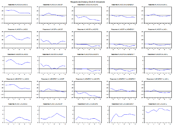
Figure-3. Impulse Responses - Turkey
Source: Graphs have been plotted by the author in EVIEWS software.
Finally, Figure 3 provides line plots of impulse responses between CO2 emissions, energy consumption, output, and oil price. As it can be seen from Figure 3, the response of CO2 emissions to given shocks in energy consumption is negative for the whole period and to oil price is positive in the second period and has downward trend in the next periods. This behavior is similar for the response of energy consumption to given shocks in oil price. In the response of GDP and squared GDP to given shocks in oil price is negative for the whole period. It is seen that the response of CO2 emissions to given shocks in GDP is positive in the first period but starts to decline after the second period which this finding is consistent with the findings in earlier sections of this paper.
5. CONCLUSION
This paper empirically investigates the oil price-induced EKC hypothesis, and therefore, the long-term equilibrium relationship and the direction of causality between oil price changes and carbon dioxide emissions through the channels of energy consumption and real income growth in the case of Turkey has been also searched. The theoretical EKC framework is taken into consideration in the empirical analysis with this respect. The results of the present study are of interest to both scholars and policy makers due to the reason that Turkey is a developing country and one of the most dynamic economies in the world, where its economy is linked with diverse energy resources, high-level urbanization, and rapid industrialization. The justification for doing this research is that oil price changes is expected to be in statistical relationship with energy consumption and carbon emissions in such a dynamic economy. Furthermore, this study is the first of its kind in the relevant literature to investigate the interaction between oil price changes and carbon emissions using the theoretical EKC framework, to the best of the author’s knowledge. The results of the present study show that oil price changes are in long term equilibrium relationship with carbon dioxide emissions in Turkey. Furthermore, oil price changes significantly and negatively influence the EKC and therefore carbon dioxide emissions in Turkey. Although oil movements negatively influence carbon emissions in Turkey, it does not exert significant effects on the EKC of Turkey since this curve is upward sloping no matter oil prices are added to the system or not. Therefore, this study could not validate the EKC hypothesis for Turkey by controlling oil price movements. To summarize, the results of this study suggest that oil price movements are not effectively observed and managed in Turkey as far as "Green Energies and Green Environment" are concerned. Similar researches can be replicated for the other countries, which experienced rapid urbanization and depend heavily on energy sector for comparison purposes.
Funding: This study received no specific financial support.
Competing Interests: The author declares that there are no conflicts of interests regarding the publication of this paper.
REFERENCES
Al-Abdulhadi, D.J., 2014. An analysis of demand for oil products in Middle East countries. International Journal of Economic Perspectives, 8(4): 5-12. View at Google Scholar
Al-Mulali, U.H., G.F. Assan, L.Y.M. Janice and B.C.S. CheNormee, 2013. Exploring the relationship between urbanization,energy consumption, and CO2 emission in MENA countries. Renewable and Sustainable Energy Reviews, 23: 107–112. View at Google Scholar | View at Publisher
Alshehry, A.S. and M. Belloumi, 2015. Energy consumption, carbon dioxide emissions and economic growth: The case of Saudi Arabia. Renewable and Sustainable Energy Reviews, 41: 237-247. View at Google Scholar | View at Publisher
Anatasia, V., 2015. The causal relationship between GDP, exports, energy consumption, and CO2 in Thailand and Malaysia. International Journal of Economic Perspectives, 9(4): 37-48. View at Google Scholar
Carrion-i-Silvestre, J.L., D. Kim and P. Perron, 2009. GLS-based unit root tests with multiple structural breaks under both the null and the alternative hypotheses. Econometric Theory, 25(6): 1754-1792. View at Google Scholar | View at Publisher
Gujarati, D.N., 2003. Basic econometrics. 4th Edn., New York: Mc Graw-Hill International.
Heidari, H., S.T. Katircioglu and L. Saeidpour, 2015. Economic growth, CO2 emissions, and energy consumption in the five ASEAN countries. International Journal of Electrical Power & Energy Systems, 64: 785-791. View at Google Scholar | View at Publisher
Henriques, I. and P. Sadorsky, 2008. Oil prices and the stock prices of alternative energy companies. Energy Economics, 30(3): 998-1010. View at Google Scholar | View at Publisher
Kaika, D. and E. Zervas, 2013. The environmental Kuznets Curve (EKC) theory-PartA: Concept,causes and the CO2 emissions case. Energy Policy, 62: 1392-1402. View at Google Scholar | View at Publisher
Kapusuzoglu, A., 2014. Causality relationships between carbon dioxide emissions and economic growth: Results from a multi-country study. International Journal of Economic Perspectives, 6: 5-15. View at Google Scholar
Kasman, A. and Y.S. Duman, 2015. CO2 emissions, economic growth, energy consumption, trade and urbanization in new EU member and candidate countries: A panel data analysis. Economic Modelling, 44: 97-103. View at Google Scholar | View at Publisher
Katircioglu, S., 2009. Revisiting the tourism-led-growth hypothesis for Turkey using the bounds test and Johansen approach for cointegration. Tourism Management, 30(1): 17-20. View at Google Scholar | View at Publisher
Katircioglu, S., 2010. International tourism, higher education, and economic growth: The case of North Cyprus. World Economy, 33(12): 1955-1972. View at Google Scholar | View at Publisher
Katircioglu, S.T., 2014. Testing the tourism-induced EKC hypothesis: The case of Singapore. Economic Modeling, 41: 383-391. View at Google Scholar | View at Publisher
Lau, L.-S., C. Chee-Keong and E. Yoke-Kee, 2014. Investigation of the environmental Kuznets Curve for carbon emissions in Malaysia: Do foreign direct investment and trade matter? Energy Policy, 68: 490–497. View at Google Scholar | View at Publisher
Liu, Y., 2009. Exploring the relationship between urbanization and energy consumption in China using ARDL (Autoregressive Distributed Lag) and FDM (Factor Decomposition Model). Energy, 34(11): 1846-1854. View at Google Scholar | View at Publisher
Luzzati, T. and M. Orsini, 2009. Investigatingtheenergy-environmental Kuznets Curve. Energy, 34(3): 291–300. View at Google Scholar
Magnani, E., 2000. The environmental Kuznets Curve, environmental protection policy and income distribution. Ecological Economics, 32(3): 431–443. View at Google Scholar | View at Publisher
Majumdar, S. and J. Parikh, 1996. Energy demand forecasts with investment constraints. Journal of Forecasting, 15(6): 459-476. View at Google Scholar | View at Publisher
Maki, D., 2012. Tests for cointegration allowing for an unknown number of breaks. Economic Modelling, 29(5): 2011-2015. View at Google Scholar | View at Publisher
Méjean, A. and C. Hope, 2013. Supplying synthetic crude oil from Canadian oil sands: A comparative study of the costs and CO2 emissions of mining and in-situ recovery. Energy Policy, Elsevier, 60: 27-40. View at Google Scholar | View at Publisher
Memis, A. and A. Kapusuzoglu, 2015. The impacts of global oil prices fluctuations on stock markets: An empirical analysis for OECD countries. International Journal of Economic Perspectives, 9(1): 80-91. View at Google Scholar
Saboori, B., S. Jamalludin and M. Saidatulakmal, 2012. Economic growth and CO2 emissions in Malaysia: A cointegrationan alysis of the environmental Kuznets Curve. Energy Policy, 51: 184–191. View at Publisher
Sadorsky, P., 2009. Renewable energy consumption, CO2 emissions and oil prices in the G7 countries. Energy Economics, 31(3): 456–462. View at Google Scholar | View at Publisher
Shahbaz, M., M. Mihai and A. Parvez, 2013. Environmental Kuznets Curve in Romania and the role of energy consumption. Renewable and Sustainable Energy Reviews, 18: 165–173. View at Google Scholar | View at Publisher
Silk, J. and F. Joust, 1997. Short and long-run elasticities in US residential electricity demand: A cointegration approach. Energy Economics, 19(4): 493–513. View at Google Scholar | View at Publisher
Stern, D.I., 2004. The rise and fall of the environmental Kuznets Curve. World Development, 32(8): 1419–1439. View at Google Scholar | View at Publisher
World Bank, 2016. World development indicators. Retrieved from http://www.worldbank.org [Accessed October 20, 2016].
| Views and opinions expressed in this article are the views and opinions of the author(s), Asian Economic and Financial Review shall not be responsible or answerable for any loss, damage or liability etc. caused in relation to/arising out of the use of the content. |