


IS EXPORT-LED GROWTH HYPOTHESIS EXIST IN SAUDI ARABIA? EVIDENCE FROM AN ARDL BOUNDS TESTING APPROACH

1,2,3Faculty of Economics and Administrative Sciences, Near East University, North Cyprus Nicosia Mersin, Turkey
ABSTRACT
The study investigates the relationship between economic growth, imports and export for Saudi Arabia by using the time series data from 1968-2014. The study employs the recently developed ARDL-bounds testing approach. The estimations of the ARDL-bounds testing approach indicated that imports, export and GDP are strongly co-integrated. The finding of the study further indicated that exports have positive impact on the economic growth in the long run. This specifies that if exports are increased by one percent the economic growth is increased by 3.39%, implying the validity of export-led growth hypothesis. The parameter of error correction term is 2.89% that represents the speed of adjustment. This implies that economic growth converges to its long run equilibrium position by 2.89% speed of adjustments via channel of imports and Exports. As the speed of adjustment is very low and it would take time to return back to the equilibrium level, that confirms the stability of the system. The reliability and validity of the estimations results are confirmed by the diagnostics tests both in short and long run. Finally, the results of the granger causality suggest, a uni-directional causality running from export to GDP, suggesting the validity of export led growth hypothesis. While another uni-directional causality has been found from imports to exports. Being the member of OPEC, Saudi Arabia exports mainly comprises of oil that exposes the economy of country to external shocks. The study suggested that Saudi Arabia needs to invest more in the non-oil sector and diversify their investment by attracting more FDI. This will cause the economic growth to increase and also be more flexible to any external shocks.
© 2017 AESS Publications. All Rights Reserved.
Keywords: GDP, Export, Import, ARDL, Saudi Arabia, ARDL, Pair-wise Granger causality.
Received: 21 November 2016/ Revised: 21 December 2016/ Accepted: 31 December 2016/ Published: 10 January 2017
Contribution/ Originality
This study contributes to the existing literature of OPEC countries by using ARDL to analyze the impact of exports and imports in Saudi Arabia covering the crisis period. This study is of its first kind to use Pair-wise granger causality that is applicable to the cointegrated series in case of Saudi Arabia.
1. INTRODUCTION
The economic growth of any country depends on exports and foreign exchange earnings that are used to promote economic development. The country can acquire technology and skilled labor that may increase the consumption of commodities that are not available locally. The relationship of export-led growth is being one of the major core of discussion among the economists. The proponent of export led growth support their arguments based on the performance of East Asian countries that have achieved a significant level of development by implementing the policies that favors export-led growth industrialization strategies.
Some of the studies are of the view that export-led growth must not necessarily be reinforced by uni-directional causality that runs from export to . But the reverse causality may also exist, in which growth is causing export. This implies that the significant rise in economic expansion may upsurge the output by making export more competitive in international markets. Thus, resulting in significant expansion of products to export internationally. Consequently it may stimulate export-led growth of a county. As a member of OPEC'S list Saudi Arabia economy heavily depends on exporting oil. The export of oil contributes a major proportion to the economy of Saudi Arabia in terms of . On other hand the significant fall in oil prices in international market have a strong impact on oil exports revenue that affects economic growth either insignificantly or significantly. This encourages us to investigate the nexus between exports and economic growth in case of Saudi Arabia. This motivates us to examine the linkage among GDP, exports and imports for a period 1968-2014. This period includes the crisis period when Saudi Arabia economy was in recession. In order to investigate the nexus between exports and economic growth, the ARDL model is used to estimate the short–run and long-run, followed by the Granger causality to determine the direction of causality, which will enable us to craft policy implications. The rest of the article is explained as. A brief literature review will be discussed in section 2. Section 3 describes the model specification and methodology. Section 4 elucidates the results and section 5 concludes the study.
2. BRIEF LITERATURE REVIEW
Numerous empirical studies have investigated whether export causes economic growth of a county or vice versa. Some empirical studies found exports, which stimulate economic growth of a country. While other suggests that economic growth induces exports. Although some of the empirical studies have found bidirectional relationship among both. However, still some studies couldn't find a relationship. The reason for different results is because of the economic nature of different countries and the time period under investigation. For instance, Rana (1985) conducted a study to analyze export-led growth for 14 Asian developing countries and found that export is positively contributing to economic growth. This finding of his study was augmented by the fact that export accelerates the economic growth. Abbas (2012) conducted a study between export and economic growth and find a co-integrating relationship using a period 1975-2010. The study findings suggested that production is causing export in long-run as well in short-run. Mishra (2011) conducted a study for India and examined the co-integration and causality among exports and growth for a period 1970-2009. The findings revealed a long-run relationship among export and economic growth. The results further indicated that exports are unable to cause economic growth but the later has caused exports.
Agrawal (2015) analyzed the export-led growth by examining the post liberalization period of India and found a bi-directional relationship between export-growth. Based on the above literature review and various studies conducted, it has been cleared that the direction of causality and relationship among the exports and economic growth is vague. Therefore this study is important to highlight the relationship between the export, import and economic growth for the period 1968-2014 including 2008 global financial crises.
3. MODEL SPECIFICATION AND METHODOLOGY
According to the empirical literature on import, export and GDP, we use import export and GDP to specify along relationship in the above mention variables. The long run relationship can be written in the form of econometric model as below.
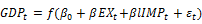 (1)
(1)
Where GDPt represents real GDP per capita (constant 2005 US$), where Ex represents exports and IMP represents imports as a percentage of GDP.  represents the error term. The data has been collected from the World Bank (2015). The sample is sufficient enough to apply the newly design ARDL technique in time series. Log-Log model is used to lessen the effect of heteroscedasticity, if there exists. After the transformation to the natural logarithms the model can be written as
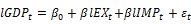 (2)
(2)
3.1. Methodology
The unit root test in the time series is to check the stationarity of the data by using different unit root test to determine the order of integration. A number of unit root tests exist to investigate the stationarity of the data. Enders (1995) recommended the use of more than one unit root test to determine the correct order of variables. Augmented Dickey and Fuller (1981) and the Phillips and Perron (1988) are the two widely unit root tests reported by numerous studies. The correct order of integration for the estimated variables can only be trusted if both the unit root test gives the same results.
3.1.1. Auto Regressive Distributed Lag (ARDL) Co-Integration
To find the relationship between exports, import and , this empirical study employed the recently developed autoregressive distributed-lag (ARDL) developed by Pesaran et al. (2001). The ARDL approach to co-integration has many advantages. Firstly, the ARDL model is flexible in terms of its application to any series whether the regressors are I(0)and/ or I(1) or mixed order of integration, provided that the dependent variable should be I(1). Secondly, this model can be better applied to determine the co-integration relationship in small samples. Thirdly, the ARDL can identify different optimal lags for different variables. The long-run co-integration among the variables in the estimated models can be determined by using Wald or F- test. Wald or F-test represents the joint significant test of the lag variables.
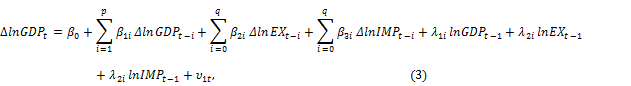
Where  is an error term that should be white noise and Δ represents the first difference. lngdp represents the gross domestic product per capita, lnex represents exports, and lnimp represents imports. The AIC criteria was used for appropriate lag selection. The joint F- statistics or Wald statistics is used to test the null hypothesis of no co-integartion among variables in equation (2) is H0: α1 = α2 = α3 = 0 tested against the alternative hypothesis H1: α1 ≠ α2 ≠ α3 ≠ 0. The estimated value of F- statistics is matched with the two sets of critical values classified as upper-bounds and lower-bounds I(1), and I(0) respectively. If the estimated value of F-statistics lies above the I(1), and I(0) critical values, then the null hypothesis of co-integration is rejected. If the estimated F-statistics values lie in between I(1), and I(0) critical values, then the decision regarding co-integration is indecisive. If the F-statistics values fall below I(1), and I(0), then the null hypothesis of no cointegration is accepted.
If the cointegration is confirmed among the variables in Equation 3, then the estimated coefficients in the long-run model and short run model can be estimated by using Equation 4, and Equation 5, that shows the short run dynamics as
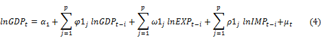
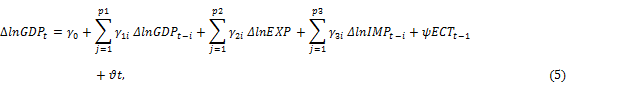
Where represents the error correction term. The sign of the ECT must be negative and statistically significant and the coefficient value should be between 0-1. The ECT represents the speed of adjustment to converge the dynamics back to the symmetry after a short run, which confirms the system stability.
3.1.2. Model Stability and Dignostic Tests
To determine the reliability and validity of the ARDL model several diagnostics and model stability tests are performed. The diagnostics tests are used to observe the normality test, the heteroscedasticity test, the residual serial correction and the correlogram of the residuals to find the presence of the auto correlation. The stability model can be checked by using CUSUM test proposed by Brown et al. (1975).
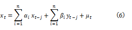
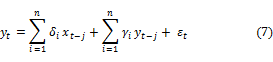
3.2. Granger Causality Test
Granger (1988) introduce a causality test, to predict how much y causes x. To find out, whether y is causing x, means that in what way significantly the present value of x can be explain better by the previous values of x and to see the effect that the explanation of x can be more improved by adding the lagged values of y. it can be concluded that x is Granger caused by y not because that x is because of y rather than x can be determined from the past values of x and y and not alone x.
The estimation of the Granger causality results based on F statistics by using AIC for appropriate lag selection.
4. EMPIRICAL RESULTS AND ANALYSIS
4.1. Unit Root Tests for Stationarity
To identify the cointegration between export growth and import it is necessary to analyze the stationarity nature of variables. The results of ADF and PP tests have been reported in Table 1 and Table 2. Both ADF and PP are used to test the stationarity nature of the variables. Schwarz information criteria were recommended for selecting the optimum lag as suggested by Pesaran and Shin (1998).
Table-1. Augmented Dickey Fuller Unit Root test results for Stationarity of variables
| Country (Sample Period) | ADF | ADF | ||
| Saudi Arabia (1968-2014) | Level | First Difference | ||
| Intercept | Intercept and Trend | Intercept | Intercept and Trend | |
| LGDP | -2.3448 (0) | -2.5613 (0) | -3.6233***(0) | -4.7822***(12) |
| LEX | -2.0268 (0) | -2.0163 (0) | -7.2453***(0) | -7.1621*** (0) |
| LIMP | -2.2489 (0) | -2.2999 (0) | -4.4799*** (2) | -4.4779*** (2) |
Note: (i) The EVeiws 9 has been used for performing the unit root tests. (ii) The Augmented Dickey Fuller unit root test was performed both at level and first differenced (intercept, and both the trend and intercept) (iii) The figures in the parenthesis represents the lags selected by using the Schwarz info criteria (SIC). (iv)*, **, *** represents significant at 10%, 5%, and 1%.
Source: Author’s own computation
Table-2. Philips Perron (PP) Unit Root test results for Stationarity of variables
| Country (Sample Period) | PP | PP | ||
| Saudi Arabia (1960-2012) | Level | First Difference | ||
| Intercept | Intercept and Trend | Intercept | Intercept and Trend | |
| LGDP | -1.8838 (4) | -2.5899 (4) | -3.6587*** (3) | -3.7935** (4) |
| LEX | -2.0133 (1) | -2.0049 (1) | -7.2414*** (2) | -7.1592***(2) |
| LIMP | -2.2665 (1) | -2.2999 (0) | -7.2559*** (5) | -7.1537*** (5) |
Note: (i) The EVeiws 9 has been used for performing the unit root tests with Newey-West using Bartlett Kernel.. (ii) The Phillips-Perron unit root test was performed both at level and first differenced (intercept, and both the trend and intercept) (iii)*, **, *** represents significant at 10%, 5%, and 1%. The figures in the parenthesis represents the lags selected by using the Schwarz info criteria (SIC).
Source: Author’s own computation
As it has been evident from both tables that all the variables in a series are non-stationary at level and become stationary by taking the first difference. Now the bounds test of cointegration can be applied to Equation 3 to determine the long run relationship among the estimated variables.
Table-3. Results of Bounds test of Co-integration.
Note: *, ** and *** represents significance level at 10%, 5%, and 1% level respectively. The AIC criterion is used to determine the optimal lag. The critical values are determined from Pesaran et al. (2001).
Source: Author’s own computation
Table 3 shows the computed F-statistics value for model. The second row of the table represents the optimum lag length, which was selected on the basis of AIC criterion. The table shows that there is a mutual long-run relationship amongst the variables. Because the computed F-statistics (23.9882) lies above the lower and upper bounds critical values by Pesaran et al. (2001) at even 1%. The long run and short-run relationship is estimated by using Equation 4 and 5.
It can be observed from Table 4, the long-run coefficient of export is positive, elastic and significant. This specifies that if exports are increased by one percent the economic growth rises by 3.39%, implying the validity of export led growth hypothesis in the long-run. At the same time the elasticity of import is negative but is highly insignificant in the long run and has no influence on economic growth. The elasticity of export in the short-run is statistically significant. This implies the validity of export-led growth hypothesis not only in long-run but also in short-run. While the coefficient of import is negative but statistically significant in the short-run. The Parameters of error correction term is 2.89% that represents the speed of adjustment. The parameter of the ECT is negative less than one and is statistically significant even at 1%. This implies that economic growth converges to its long run equilibrium position by 2.89% speed of adjustments via channel of imports and Exports.
Table-4. ARDL Long run and short run results
| Dependent Variable: LnGDPt | |||
| Long-run results | |||
| Variable | Coefficient | Standard Error | t-Statistics |
| Constant | 16.3436 | 5.6783 | 2.8782*** |
| LnEXP | 3.3932 | 1.7697 | 1.9173* |
| LnIMP | -0.0548 | 0.0511 | -1.0724 |
| R2 | 0.99 | S.E of regression. | 0.0389 |
| Adj. R2 | 0.99 | Sum Squared resid | 0.0575 |
| F-Statistics | 947.6946*** | DW | 1.65 |
| Short-run results | |||
| Variable | Coefficient | Standard Error | t-Statistics |
| Constant | 0.4735 | 0.3550 | 1.3339 |
| ∆lnEXP | 0.1380 | 0.0353 | 3.9032*** |
| ∆lnEXPt-1 | 0.1330 | 0.0368 | 3.6135*** |
| ∆lnIMP | -0.0047 | 0.0012 | -3.7186*** |
| ECMt-1 | -0.0289 | 0.0028 | -10.1732*** |
| R2 | 0.69 | S.E of regression. | 0.0379 |
| Adj. R2 | 0.66 | Sum Squared resid | 0.0576 |
| F-Statistics | 22.3699*** | DW | 1.65 |
Note: *, ** and *** represents significance level at 10%, 5%, and 1% level respectively.
Source: Author’s own computation
As the speed of adjustment is very low, it would take time to return back to the equilibrium level, that confirms the stability of the system. The reliability and validity of the estimations results are confirmed by the diagnostics tests. Our estimations pass all the diagnostic tests both in short-run and long-run and verifying all the basic assumption of classical linear regression model that is necessary for the validity of our estimations.
Table-5. Diagnostic Tests (Long run)
| Diagnostic Test | x2SC | x2W | x2H | x2N | x2AR | Ramsey Reset Test |
| Saudi Arabia | 4.0599(0.1313) | 20.8357(0.7939) | 7.0640(0.3150) | 2.7968(0.2469) | 0.0219(0.8822) | 1.6786(0.2031) |
Note: are the test for serial correlation, White test and Breusch Pagan Godfrey test for heteroscedasticity , normality , and Arch tests for heteroscedasticity. The numbers in the brackets is the P-Values. Ramsey Reset test was performed by taking the F-statistics.
Source: Author’s own computation
Table-6. Diagnostic Tests (Short run)
| Diagnostic Test | x2SC | x2W | x2H | x2N | x2AR | Ramsey Reset Test |
| Saudi Arabia | 3.8266(0.1476) | 13.6168(0.4786) | 4.111(0.3911) | 2.7968(0.2469) | 0.02195(0.8822) | 0.2963(0.5893) |
Note: are the test for serial correlation, White test and Breusch Pagan Godfrey test for heteroscedasticity , normality , and Arch tests for heteroscedasticity. The numbers in the brackets is the P-Values. Ramsey Reset test was performed by taking the F-statistics.
Source: Author’s own computation
4.2. CUSUM and CUSUMQ Test Results
The estimated ARDL, with AIC based criterion error correction model is implemented to apply the CUSUM and CUSUMQ stability tests. Both the graphs of the CUSUM and CUSUMQ have been given in figure 1 and figure 2. As both the plots of CUSUM and CUSUMQ statistics fall inside the critical bounds, that indicates that the estimated coefficients of the error correction model are stable over a period of time from 1968-2014.
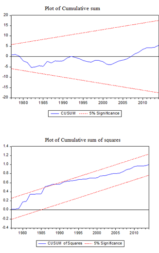
Figure-1. The estimated blue-line is within the 5% significance level, implying the stability of the model for a period 1968-2014.
Source: Author’s own computation
4.3. Pair Wise Granger Causality Test
The result of the granger causality tests has been reported in table 7. In order to conserve the space only the significant results are displayed in table 7. The AIC was used to select the lag. The Granger causality test is used to craft suitable policy by predicting the direction of causality. The results showed a unidirectional causality that runs from exports to GDP. This means that export is causing GDP or in other words it is because of the export that stimulates growth in Saudi Arabia for a period 1968-2014. The unidirectional causality from export to GDP corroborates the Export-led growth hypothesis which is in concordance with the long-run and short-run results of ARDL bounds testing approach. The empirical results of our study have been consistent with the studies conducted by El-Sakka and Al-Mutairi (2000). While a uni-directional causality has been found from imports to exports, while on other side exports are causing GDP. That means that import is indirectly causing GDP.
Table-7. Results of pair wise Granger2 Causality Test.
| Null hypothesis | F-Statistics | P-Value | implication |
| D(LEX) does not granger cause D(LGDP) | 11.8233*** | 0.0013 | LEX is causing GDP |
| D(LIMP) does not granger cause D(LEX) | 3.3357* | 0.0749 | LIMP is causing LEX |
Note: ***,*represents 1% and 10% significance level. The lag selection was done by using the AIC.a .
Source: Author’s own computation
5. CONCLUSION AND POLICY IMPLICATION
The study investigates the relationship between economic growth, imports and export for Saudi Arabia by using the time series data from 1968-2014. The study employs the recently developed ARDL-bounds testing approach. The estimations of the ARDL-bounds testing approach indicated that imports, export and GDP are strongly co-integrated. This implies that there is a long run relationship among the variables. The finding of the study further indicated that exports have positive impact on the economic growth in the long run. This specifies that if exports are increased by one percent the economic growth is increased by 3.39%, implying the validity of export led growth hypothesis. At the same time the elasticity of import is negative but is highly insignificant in the long run and has no influence on economic growth. The Parameters of error correction term is 2.89% that represents the speed of adjustment. This implies that economic growth converges to its long run equilibrium position by 2.89% speed of adjustments via channel of imports and Exports. As the speed of adjustment is very low and it would take time to return back to the equilibrium level, that confirms the stability of the system. The reliability and validity of the estimations results are confirmed by the diagnostics tests. Finally, the results of the granger causality suggest, a uni-directional causality running from export to GDP, suggesting the validity of export led growth hypothesis. While a uni-directional causality has been found from imports and exports, and exports are causing GDP.
The oil is the main source of revenue generation for Saudi Arabia in terms of its export to other countries. Being the member of OPEC, Saudi Arabia exports mainly comprises of oil that exposes the economy of country to external shocks. This has been quite evident during the recession in the year 2008-09 by the sharp declined in the oil price. The Saudi Arabia was having negative exports and the GDP was stagnant after 2008-09 oil shock. The study suggested that Saudi Arabia needs to invest more in the non-oil sector and diversify their investment by attracting more FDI. This will cause the economic growth to increase and also be more flexible to any external shocks. The prospect study in this regard can further be conducted by including more relevant variables as FDI, real exchange rate that can be used as the determinants of GDP in case of Saudi Arabia.
| Funding: This study received no specific financial support. |
| Competing Interests: The authors declare that they have no competing interests. |
| Contributors/Acknowledgement: All authors contributed equally to the conception and design of the study. |
REFERENCES
Abbas, S., 2012. Causality between exports and economic growth: Investigating suitable trade policy for Pakistan. Eurasian Journal of Business and Economics, 5(10): 91-98. View at Google Scholar
Agrawal, P., 2015. The role of exports in India's economic growth. Journal of International Trade & Economic Development, 24(6): 835-859. View at Google Scholar | View at Publisher
Brown, R.L., J. Durbin and J.M. Evans, 1975. Techniques for testing the constancy of regression relationships over time. Journal of the Royal Statistical Society, 37(2): 149-192. View at Google Scholar
Dickey, D. and W.A. Fuller, 1981. Likelihood ratio statistics for autoregressive time series with a unit root. Econometrica, 49(4): 1057-1072. View at Google Scholar | View at Publisher
El-Sakka, M.I. and N.H. Al-Mutairi, 2000. Exports and economic growth: The Arab experience. Pakistan Development Review, 9(2): 153-169. View at Google Scholar
Enders, W., 1995. Applied econometric time series. 3rd Edn., New York: John Wiley & Sons Inc.
Granger, C.W.J., 1988. Causality, cointegration, and control. Journal of Economic Dynamics and Control, 12(2-3): 551-559. View at Google Scholar | View at Publisher
Mishra, P.K., 2011. The dynamics of relationship between exports and economic growth in India. International Journal of Economic Sciences and Applied Research, 4(2): 53-70. View at Google Scholar
Pesaran, M.H. and Y. Shin, 1998. An autoregressive distributed-lag modelling approach to cointegration analysis. Econometric Society Monographs, 31: 371-413. View at Google Scholar | View at Publisher
Pesaran, M.H., Y. Shin and R.J. Smith, 2001. Bounds testing approaches to the analysis of level relationships. Journal of Applied Econometrics, 16(3): 289–326. View at Google Scholar | View at Publisher
Phillips, P.C.B. and P. Perron, 1988. Testing for a unit root in time series regression. Biometrika, 75(2): 335–346. View at Google Scholar | View at Publisher
Rana, P.B., 1985. Exports and economic growth in the Asian region (No. 25). The Bank.
World Bank, 2015. World development indicators. Retrieved from http://www.worldbank.org.
| Views and opinions expressed in this article are the views and opinions of the author(s), Asian Journal of Economic Modelling shall not be responsible or answerable for any loss, damage or liability etc. caused in relation to/arising out of the use of the content. |