


THE VOLATILITY STRUCTURE OF GLOBAL FINANCIAL MARKETS: A COMPARATIVE ANALYSIS

1,2Institute for Financial Management and Research, Nungambakkam, Chennai, India
ABSTRACT
The study is basically an extension of the k-day Vol ratio analysis on Nifty Index, proposed by Viswanathan and Maheswaran (2016). It examines the impact of the global financial crisis of 2008 on the structure of volatility of global indices (S&P500, FTSE100 and DAX). The global indices did not experience a significant change in volatility structure. On comparison, the behavior of volatility of NIFTY index subsequent to the financial crisis is found to be similar to that of global indices. The present study indicates that due to the crisis, NIFTY has joined the league of developed capital markets with respect to the structure of volatility.
© 2017 AESS Publications. All Rights Reserved.
Keywords: Volatility of volatility, Long memory, Financial crisis, Vol ratio, Global indices, Structure of volatility.
JEL Classification: G01, G10, G19.
Received: 23 November 2016/ Revised: 16 December 2016/ Accepted: 30 December 2016/ Published: 7 January 2017
Contribution/ Originality
The paper contributes the first logical analysis of change in structure of volatility of the global indices due to the financial crisis of 2008 by making use of a novel estimator called Vol ratio that is put forward by Viswanathan and Maheswaran (2016).
1. INTRODUCTION
Long memory dynamics is an extensively investigated phenomenon. The presence of long memory or long-range dependence has important implications as traditional theories are built on the assumption of independently and identically distributed stock returns (Mandelbrot, 1971). The study of long-memory aids in examining the structure of volatility in stock returns. Breidt et al. (1998); Baillie et al. (1996); Ding and Granger (1996); Comte and Renault (1998) and Robinson (1991;2001) found evidence for long memory in realized volatility. Analyzing the structure of volatility reveals immense information regarding financial markets and helps in forming better trading strategies. Researchers are keen to examine the impact of various events on the structure of volatility (Click and Plummer, 2005; Lim et al., 2008). The global financial crisis of 2008 is one such event that has been studied extensively to investigate its impact on the global stock markets and economy.
After a silent start, 2008 exploded into a financial earthquake. Since then, there has been a number of studies regarding how the global financial crisis of 2008 altered the structure of stock markets around the world. We are particularly interested in extending our previous study about the impact of the financial crisis of 2008 on the Nifty index (Viswanathan and Maheswaran, 2016) to global stock indices. This paper analyses the structure of volatility of Nifty Index by proposing a new statistic, Vol Ratio which allows to infer the behavior of volatility of volatility at various horizons. It was found that there has been a dramatic change in the structure of volatility due to the global financial crisis of 2008. In short, the volatility of volatility displays a rapid decline with respect to the horizon, whereas it does not die down subsequent to the crisis.
In this paper, we extend the analysis of the k-day Vol Ratio, proposed in the above-mentioned paper to global stock indices. We conjecture that the global stock indices will behave similar to that of Nifty Index during the post-crisis period (Figure 3). We analyze global indices such as S&P500, FTSE100 and DAX to see whether or not they have undergone any structural change due to the financial crisis of 2008. What we find is that, these indices experienced persistent and positive Vol of vol, even for longer term returns thereby indicating presence of stochastic volatility which implies long memory. Analysis on all the samples under consideration produced results similar to that of Nifty index during post-crisis period.
The rest of the paper is organized in 4 sections. Section 2 consists of an extensive literature review. Section 3, Methodology has two sub-sections namely 3.1 summarizes theory and 3.2 describes the model. Section 4 contains details of empirical analysis with separate sub-sections for data (4.1), analysis (4.2) and empirical findings (4.3). Section 5 contains concluding remarks.
2. LITERATURE REVIEW
In finance, long memory has a long history and continues to be a topic of active research. Mandelbrot (1971) was among the first to consider the effect of persistent dependence in asset prices. He argued that martingale and random walk models of speculative prices may not be reliable in the presence of long-range dependence. This observation was followed by a number of empirical studies focused on examining the long-range dependence in asset prices as well as the development of various methods of estimation of long memory.
Stochastic models that exhibit dependence over very long time spans such as fractionally integrated time series models of Mandelbrot and Van (1968); Granger and Joyeux (1980) and Hosking (1981) were introduced. These processes have an auto-correlation function that decays slowly than the short-term dependent time series. Bollerslev (1986) proposed the Generalized autoregressive conditional heteroscedasticity (GARCH) model to detect long-range dependence. Lo and MacKinlay (1988) made use of the ratio of the variance of k-week stock returns to k times the variance of one-week stock returns. They found that the ratio goes above unity for small values of k (2≤ k ≤32). Poterba and Summers (1988) pointed out that the variance ratio falls below one for much larger values of k.
Among other methods of detecting long-range dependence, the classical R/S statistic developed by Hurst (1951) is of great significance. Mandelbrot (1972) demonstrated the superiority of R/S analysis. This method was further augmented by Lo (1989) as modified R/S analysis. Variations of GARCH model such as IGARCH (Nelson, 1990); EGARCH (Nelson, 1991) NGARCH (Higgins and Bera, 1992) QGARCH (Sentana, 1995) TGARCH (Zakoian, 1994) GJR GARCH (Glosten et al., 1993) FIGARCH (Baillie et al., 1996) CO-GARCH (Klüppelberg et al., 2004) etc. emerged later.
In light of these methods, a number of studies substantiating the evidence of long memory in stock returns were undertaken. Ding et al. (1993); Bollerslev and Mikkelsen (1996); Mikosch and Starica (1998) analyzed S&P 500 and found evidence for long-range dependence. Some of the recent studies such as Granger and Hyung (2004) and Heyde and Yang (2010) supports the existence of long memory in American stock market.
There is plenty of research regarding long memory in European stock markets. Di Matteo et al. (2005) made use of generalized Hurst approach for establishing the presence of long-range dependence in the U.K stock returns. Granero et al. (2008) used R/S analysis to arrive at the same conclusion. Cheung and Lai (1995); Jacobsen (1996); Cajueiro and Tabak (2008) verified the presence of long memory for other European markets using modified R/S and R/S analysis.
Long memory dynamics in global stock markets has been analyzed using various methods. Our contribution in this paper is to document long-memory effects in global stock markets by making use of the novel method that was put forward by Viswanathan and Maheswaran (2016).
3. METHODOLOGY
3.1. Theory
The key variable used for the analysis is the daily log returns which is defined as,
xt = ln (Closing index level on day t) – ln (Closing index level on day t-1)
We assume that the unconditional distribution of the stock returns follow a mixture of normal distributions as in the context of the Mixture of Distribution Hypothesis (Clark, 1973). That is to say,
xt = Zt 
Where, Yt is stochastic variance on day t
Zt is the standard normal variable.
The statistic considered for the analysis is Vol Ratio, which is defined as,
Vol Ratio = 
= 
= E [ ] {when xt is normalized)
To observe the variation of volatility on day t, we consider the statistic, Vol of vol.
Vol of vol = 
= 
The statistics used in our analysis are Vol Ratio and Vol of vol. There is evidence of deviation from normality if Vol Ratio is less than unity. The stochastic nature of volatility can be confirmed if the Vol of vol turns out to be significantly higher than zero.
3.2. Model
We follow the model proposed by Viswanathan and Maheswaran (2016). The series of k-day returns is generated using the following formula.
St(k) =  t-j
t-j
Where, xt is the daily log return,
t is number of days,
k is the number of observations to be summed up (as a moving window).
The series is then standardized using the formula:
St(k)* = (St(k) - µ*) / σ* (µ* and σ* are the sample mean and sample standard deviation
of St(k) respectively)
We then compute the Vol ratio and Vol of vol using the following formulae.
Vol Ratio = E (│ St(k)*│) / 2 ϕ(0)
Vol of vol =
In order to check for deviation from normality, it has to be tested whether or not Vol Ratio is equal to unity. The hypothesis that we are testing for each index is:
H0 : Vol Ratio = 1
Ha: Vol Ratio ≠ 1
If, Vol Ratio = 1 then, Vol of vol = 0 thus indicating the non-stochastic nature of volatility.
4. EMPIRICAL ANALYSIS
4.1. Data
Daily data of S&P500 (The United States of America), FTSE100 (The United Kingdom) and DAX (Germany) Index from Jan 1996 to February 2016 is used. The sample is further divided into 2 sub samples: Sub Sample #1 – Jan 1996 to Dec 2007 and Sub Sample #2 – Jan 2009 to February 2016. The source of data is Bloomberg.
4.2. Analysis
We follow the k-day analysis in which the data is analysed over k-day moving windows. That is to say, when k = 1, we consider the original series of daily return and when k = 3, observations (1,2,3), (2,3,4), (3,4,5) etc. are summed up to form a new series of k-day returns. Starting with the original series of daily log returns, we generate k-day series up to k = 20. The statistics, Vol Ratio and Vol of vol is calculated for each series of k-day returns. We analyse sub-sample #1 (Jan 1996 to Dec 2007) and sub-sample #2 (Jan 2009 to Dec 2015) of each index separately. To avoid ambiguity, the sub-samples are named along with the title of the indices.
4.3. Empirical Findings
The following seven tables summarize the output of the empirical analysis. Each table consists of six columns that represent width of k day window, the actual Vol Ratio, bootstrap mean and bootstrap standard error of Vol Ratio, t-statistic with respect to 1 and p-value respectively (The bootstrap technique has been made use of in order to get reliable standard errors based on the finite sample distribution of the test statistics.) Table 7 summarizes Vol of vol during sub-sample #1 and sub-sample #2. This table contain six columns representing Vol of vol of S&P500, FTSE100 and DAX respectively during each sample periods.
To test the hypothesis stated in Section 3.2, for S&P500 during sub-sample #1, we perform t-tests, with 95%confidence level. For S&P500 during sub-sample #1 (Table 1), Vol Ratio increases as k-day goes from 1 to 20. The t-stat is significant for all k-day indicating thereby that we cannot accept the null hypothesis of Vol Ratio equal to one. Vol Ratio is below one in all cases. Therefore, the null hypothesis is rejected in case of sub-sample #1 of S&P500 index.
The tests on sub-sample #2 (Table 2) of S&P500 index, indicate that Vol Ratio increases as k-day increases. The t-stat remains significant throughout, which means that the null hypothesis has to be rejected in case of stock returns of S&P500 during sub-sample #2 as well. This suggests that Vol of vol remain positive and persistent throughout both pre-crisis and post-crisis period (Table 9 and Table 10). Figure 1
Table-1. The k-day Vol Ratio of stock returns of S&P500 during the sub-sample#1 (Jan 1996 to Dec 2007)
| k day | Actual | Boot Mean | Boot Sigma | t w.r.t Boot Mean | t w.r.t 1 | p-value |
| 1 | 0.9093 | 0.9095 | 0.0092 | -0.0219 | -9.8652 | 0.0000 |
| 2 | 0.9302 | 0.9488 | 0.0083 | -2.2451 | -8.4148 | 0.0000 |
| 3 | 0.9319 | 0.9640 | 0.0085 | -3.7579 | -7.9759 | 0.0000 |
| 4 | 0.9423 | 0.9723 | 0.0085 | -3.5054 | -6.7571 | 0.0000 |
| 5 | 0.9409 | 0.9772 | 0.0091 | -3.9676 | -6.4672 | 0.0000 |
| 6 | 0.9404 | 0.9810 | 0.0094 | -4.3177 | -6.3415 | 0.0000 |
| 7 | 0.9371 | 0.9838 | 0.0097 | -4.7984 | -6.4615 | 0.0000 |
| 8 | 0.9349 | 0.9869 | 0.0098 | -5.2934 | -6.6283 | 0.0000 |
| 9 | 0.9352 | 0.9884 | 0.0105 | -5.0539 | -6.1540 | 0.0000 |
| 10 | 0.9383 | 0.9896 | 0.0106 | -4.8552 | -5.8416 | 0.0000 |
| 11 | 0.9422 | 0.9908 | 0.0110 | -4.4239 | -5.2560 | 0.0000 |
| 12 | 0.9447 | 0.9920 | 0.0106 | -4.4638 | -5.2240 | 0.0000 |
| 13 | 0.9503 | 0.9934 | 0.0117 | -3.6796 | -4.2426 | 0.0000 |
| 14 | 0.9534 | 0.9947 | 0.0113 | -3.6591 | -4.1317 | 0.0000 |
| 15 | 0.9537 | 0.9951 | 0.0123 | -3.3574 | -3.7527 | 0.0002 |
| 16 | 0.9523 | 0.9962 | 0.0127 | -3.4527 | -3.7499 | 0.0002 |
| 17 | 0.9514 | 0.9968 | 0.0126 | -3.5848 | -3.8409 | 0.0001 |
| 18 | 0.9516 | 0.9971 | 0.0127 | -3.5956 | -3.8214 | 0.0001 |
| 19 | 0.9528 | 0.9969 | 0.0137 | -3.2319 | -3.4581 | 0.0005 |
| 20 | 0.9548 | 0.9984 | 0.0135 | -3.2349 | -3.3508 | 0.0008 |
Notes to Table 1: This table displays the k-day Vol Ratio of stock returns of S&P500 index during sub-sample #1 (Jan 1996 to Dec 2007). Boot mean indicates mean of Vol Ratio computed from bootstrap samples (generated in MATLAB) for each k-day. Bootstrap standard errors are given in column 4. The t-statistic with respect to 1 and p-value are also given.
Table-2. The k-day Vol Ratio of stock returns of S&P500 during the sub-sample#2 (Jan 2009 to Feb 2016)
| k day | Actual | Boot Mean | Boot Sigma | t w.r.t Boot Mean | t w.r.t 1 | p-value |
| 1 | 0.8628 | 0.8628 | 0.0116 | -0.0057 | -11.8434 | 0.0000 |
| 2 | 0.8991 | 0.9232 | 0.0117 | -2.0595 | -8.6115 | 0.0000 |
| 3 | 0.9032 | 0.9473 | 0.0110 | -3.9948 | -8.7734 | 0.0000 |
| 4 | 0.9134 | 0.9604 | 0.0115 | -4.0774 | -7.5173 | 0.0000 |
| 5 | 0.9009 | 0.9681 | 0.0124 | -5.4408 | -8.0206 | 0.0000 |
| 6 | 0.9004 | 0.9742 | 0.0122 | -6.0534 | -8.1647 | 0.0000 |
| 7 | 0.9007 | 0.9783 | 0.0122 | -6.3463 | -8.1162 | 0.0000 |
| 8 | 0.8949 | 0.9812 | 0.0139 | -6.2038 | -7.5581 | 0.0000 |
| 9 | 0.8952 | 0.9850 | 0.0130 | -6.9103 | -8.0677 | 0.0000 |
| 10 | 0.9010 | 0.9874 | 0.0139 | -6.2310 | -7.1415 | 0.0000 |
| 11 | 0.8985 | 0.9888 | 0.0147 | -6.1590 | -6.9266 | 0.0000 |
| 12 | 0.9030 | 0.9909 | 0.0142 | -6.1700 | -6.8125 | 0.0000 |
| 13 | 0.9020 | 0.9917 | 0.0148 | -6.0702 | -6.6356 | 0.0000 |
| 14 | 0.8971 | 0.9923 | 0.0158 | -6.0275 | -6.5128 | 0.0000 |
| 15 | 0.9012 | 0.9938 | 0.0160 | -5.7974 | -6.1879 | 0.0000 |
| 16 | 0.9054 | 0.9953 | 0.0162 | -5.5617 | -5.8499 | 0.0000 |
| 17 | 0.9041 | 0.9966 | 0.0166 | -5.5840 | -5.7862 | 0.0000 |
| 18 | 0.9012 | 0.9981 | 0.0172 | -5.6283 | -5.7366 | 0.0000 |
| 19 | 0.9048 | 0.9987 | 0.0174 | -5.3946 | -5.4717 | 0.0000 |
| 20 | 0.9104 | 0.9996 | 0.0174 | -5.1271 | -5.1515 | 0.0000 |
Notes to Table 2: This table displays the k-day Vol Ratio of stock returns of S&P500 index during the Sub-sample #2 (Jan 2009 to Feb 2016). Boot mean indicates mean of Vol-Ratio computed from bootstrap samples (generated in MATLAB) for each k-day. Bootstrap standard errors are given in column 4. The t-statistic with respect to 1 and p-value are also given.
The t-test on returns of FTSE100 index during sub Sample #1 (Table 3) shows that Vol Ratio is significantly less than unity. Therefore Vol of vol remains positive indicating that the volatility of long-term return is stochastic during this period. The result of t-test is similar in case of returns of FTSE100 during sub-sample #2 (Table 4). The null hypothesis of Vol Ratio equal to one is rejected in both cases. We can say that, volatility is persistent and does not die down during the pre-crisis as well as post-crisis period for FTSE100 index.
Table-3. The k-day Vol Ratio of stock returns of FTSE100 during the sub-sample#1 (Jan 1996 to Dec 2007)
| k day | Actual | Boot Mean | Boot Sigma | t w.r.t Boot Mean | t w.r.t 1 | p-value |
| 1 | 0.9076 | 0.9077 | 0.0076 | -0.0249 | -12.1211 | 0.0000 |
| 2 | 0.9152 | 0.9470 | 0.0076 | -4.1837 | -11.1308 | 0.0000 |
| 3 | 0.9145 | 0.9634 | 0.0073 | -6.7311 | -11.7586 | 0.0000 |
| 4 | 0.9195 | 0.9728 | 0.0078 | -6.8226 | -10.3059 | 0.0000 |
| 5 | 0.9181 | 0.9785 | 0.0084 | -7.2017 | -9.7716 | 0.0000 |
| 6 | 0.9243 | 0.9829 | 0.0090 | -6.5191 | -8.4196 | 0.0000 |
| 7 | 0.9268 | 0.9858 | 0.0091 | -6.4587 | -8.0204 | 0.0000 |
| 8 | 0.9247 | 0.9878 | 0.0094 | -6.7026 | -7.9930 | 0.0000 |
| 9 | 0.9246 | 0.9897 | 0.0101 | -6.4352 | -7.4506 | 0.0000 |
| 10 | 0.9206 | 0.9903 | 0.0105 | -6.6435 | -7.5713 | 0.0000 |
| 11 | 0.9214 | 0.9925 | 0.0106 | -6.7023 | -7.4094 | 0.0000 |
| 12 | 0.9217 | 0.9931 | 0.0113 | -6.3251 | -6.9380 | 0.0000 |
| 13 | 0.9276 | 0.9943 | 0.0113 | -5.8799 | -6.3838 | 0.0000 |
| 14 | 0.9318 | 0.9954 | 0.0110 | -5.7560 | -6.1768 | 0.0000 |
| 15 | 0.9324 | 0.9962 | 0.0120 | -5.3210 | -5.6367 | 0.0000 |
| 16 | 0.9285 | 0.9967 | 0.0123 | -5.5546 | -5.8262 | 0.0000 |
| 17 | 0.9270 | 0.9975 | 0.0123 | -5.7475 | -5.9502 | 0.0000 |
| 18 | 0.9231 | 0.9972 | 0.0130 | -5.6833 | -5.8992 | 0.0000 |
| 19 | 0.9247 | 0.9985 | 0.0124 | -5.9275 | -6.0499 | 0.0000 |
| 20 | 0.9280 | 0.9986 | 0.0137 | -5.1653 | -5.2698 | 0.0000 |
Notes to Table 3: This table displays the k-day Vol Ratio of stock returns of FTSE100 index during the Sub-sample #1 (Jan 1996 to Dec 2007). Boot mean indicates mean of Vol-Ratio computed from bootstrap samples (generated in MATLAB) for each k-day. Bootstrap standard errors are given in column 4. The t-statistic with respect to 1 and p-value are also given.
Table-4. The k-day Vol Ratio of stock returns of FTSE100 during the sub-sample#2 (Jan 2009 to Feb 2016)
| k day | Actual | Boot Mean | Boot Sigma | t w.r.t Boot Mean | t w.r.t 1 | p-value |
| 1 | 0.9083 | 0.9092 | 0.0090 | -0.1033 | -10.1472 | 0.0000 |
| 2 | 0.9246 | 0.9513 | 0.0092 | -2.9072 | -8.2263 | 0.0000 |
| 3 | 0.9276 | 0.9684 | 0.0094 | -4.3122 | -7.6602 | 0.0000 |
| 4 | 0.9336 | 0.9765 | 0.0100 | -4.3123 | -6.6691 | 0.0000 |
| 5 | 0.9289 | 0.9819 | 0.0104 | -5.1150 | -6.8629 | 0.0000 |
| 6 | 0.9306 | 0.9860 | 0.0111 | -4.9792 | -6.2387 | 0.0000 |
| 7 | 0.9281 | 0.9886 | 0.0112 | -5.3927 | -6.4070 | 0.0000 |
| 8 | 0.9273 | 0.9908 | 0.0117 | -5.4178 | -6.2075 | 0.0000 |
| 9 | 0.9367 | 0.9926 | 0.0123 | -4.5494 | -5.1496 | 0.0000 |
| 10 | 0.9426 | 0.9941 | 0.0125 | -4.1202 | -4.5965 | 0.0000 |
| 11 | 0.9433 | 0.9954 | 0.0129 | -4.0313 | -4.3903 | 0.0000 |
| 12 | 0.9459 | 0.9959 | 0.0137 | -3.6383 | -3.9401 | 0.0001 |
| 13 | 0.9465 | 0.9967 | 0.0145 | -3.4576 | -3.6829 | 0.0002 |
| 14 | 0.9505 | 0.9980 | 0.0150 | -3.1624 | -3.2974 | 0.0010 |
| 15 | 0.9492 | 0.9989 | 0.0148 | -3.3561 | -3.4330 | 0.0006 |
| 16 | 0.9492 | 1.0004 | 0.0156 | -3.2932 | -3.2656 | 0.0011 |
| 17 | 0.9478 | 1.0009 | 0.0161 | -3.2982 | -3.2417 | 0.0012 |
| 18 | 0.9459 | 1.0007 | 0.0166 | -3.2934 | -3.2502 | 0.0012 |
| 19 | 0.9508 | 1.0018 | 0.0169 | -3.0248 | -2.9178 | 0.0035 |
| 20 | 0.9524 | 1.0026 | 0.0172 | -2.9253 | -2.7729 | 0.0056 |
Notes to Table 4: This table displays the k-day Vol Ratio of stock returns of FTSE100 index during the Sub-sample #2 (Jan 2009 to Feb 2016). Boot mean indicates mean of Vol-Ratio computed from bootstrap samples (generated in MATLAB) for each k-day. Bootstrap standard errors are given in column 4. The t-statistic with respect to 1 and p-value are also given.
Sub-sample #1 (Table 5) and sub-sample #2 (Table 6) of DAX displays results that are in agreement with the results of the t-tests conducted for the sub-samples of S&P500 and FTSE100. That is to say, the samples prior and after the global financial crisis experiences increasing Vol Ratio as k-day goes from 1 to 20. Vol of vol for all k-day remain positive thereby indicating the presence of stochastic volatility in long-term returns. The null hypothesis of Vol Ratio = 1 can be rejected for this sub-sample as well at 95% confidence interval.
Table-5. The k-day Vol Ratio of stock returns of DAX during the sub-sample#1 (Jan 1996 to Dec 2007)
| k day | Actual | Boot Mean | Boot Sigma | t w.r.t Boot Mean | t w.r.t 1 | p-value |
| 1 | 0.8980 | 0.8984 | 0.0083 | -0.0488 | -12.3202 | 0.0000 |
| 2 | 0.9032 | 0.9440 | 0.0075 | -5.4736 | -12.9848 | 0.0000 |
| 3 | 0.9135 | 0.9605 | 0.0078 | -6.0184 | -11.0781 | 0.0000 |
| 4 | 0.9128 | 0.9700 | 0.0082 | -6.9992 | -10.6620 | 0.0000 |
| 5 | 0.9209 | 0.9760 | 0.0087 | -6.3127 | -9.0651 | 0.0000 |
| 6 | 0.9255 | 0.9804 | 0.0091 | -6.0635 | -8.2206 | 0.0000 |
| 7 | 0.9246 | 0.9837 | 0.0096 | -6.1752 | -7.8833 | 0.0000 |
| 8 | 0.9250 | 0.9860 | 0.0101 | -6.0331 | -7.4141 | 0.0000 |
| 9 | 0.9251 | 0.9884 | 0.0102 | -6.2388 | -7.3786 | 0.0000 |
| 10 | 0.9244 | 0.9891 | 0.0104 | -6.2060 | -7.2507 | 0.0000 |
| 11 | 0.9179 | 0.9903 | 0.0108 | -6.7013 | -7.5996 | 0.0000 |
| 12 | 0.9159 | 0.9915 | 0.0105 | -7.1725 | -7.9762 | 0.0000 |
| 13 | 0.9164 | 0.9939 | 0.0113 | -6.8356 | -7.3720 | 0.0000 |
| 14 | 0.9210 | 0.9940 | 0.0114 | -6.4281 | -6.9545 | 0.0000 |
| 15 | 0.9245 | 0.9957 | 0.0121 | -5.8753 | -6.2302 | 0.0000 |
| 16 | 0.9250 | 0.9953 | 0.0121 | -5.8166 | -6.2074 | 0.0000 |
| 17 | 0.9250 | 0.9961 | 0.0128 | -5.5590 | -5.8630 | 0.0000 |
| 18 | 0.9270 | 0.9971 | 0.0130 | -5.3721 | -5.5949 | 0.0000 |
| 19 | 0.9284 | 0.9970 | 0.0129 | -5.3209 | -5.5505 | 0.0000 |
| 20 | 0.9312 | 0.9981 | 0.0142 | -4.7274 | -4.8589 | 0.0000 |
Notes to Table 5: This table displays the k-day Vol Ratio of stock returns of DAX index during the Sub-sample #1 (Jan 1996 to Dec 2007). Boot mean indicates mean of Vol-Ratio computed from bootstrap samples (generated in MATLAB) for each k-day. Bootstrap standard errors are given in column 4. The t-statistic with respect to 1 and p-value are also given.
Table-6. The k-day Vol Ratio of stock returns of DAX during the sub-sample#2 (Jan 2009 to Feb 2016)
| k day | Actual | Boot Mean | Boot Sigma | t w.r.t Boot Mean | t w.r.t 1 | p-value |
| 1 | 0.9120 | 0.9126 | 0.0086 | -0.0769 | -10.1924 | 0.0000 |
| 2 | 0.9341 | 0.9581 | 0.0082 | -2.9201 | -8.0267 | 0.0000 |
| 3 | 0.9343 | 0.9733 | 0.0091 | -4.2701 | -7.1943 | 0.0000 |
| 4 | 0.9352 | 0.9812 | 0.0095 | -4.8486 | -6.8310 | 0.0000 |
| 5 | 0.9382 | 0.9854 | 0.0101 | -4.6884 | -6.1337 | 0.0000 |
| 6 | 0.9396 | 0.9894 | 0.0106 | -4.6898 | -5.6882 | 0.0000 |
| 7 | 0.9356 | 0.9914 | 0.0106 | -5.2415 | -6.0507 | 0.0000 |
| 8 | 0.9326 | 0.9934 | 0.0115 | -5.2662 | -5.8391 | 0.0000 |
| 9 | 0.9367 | 0.9943 | 0.0122 | -4.7106 | -5.1810 | 0.0000 |
| 10 | 0.9378 | 0.9957 | 0.0123 | -4.7057 | -5.0510 | 0.0000 |
| 11 | 0.9419 | 0.9965 | 0.0130 | -4.1822 | -4.4529 | 0.0000 |
| 12 | 0.9433 | 0.9979 | 0.0132 | -4.1442 | -4.3001 | 0.0000 |
| 13 | 0.9470 | 0.9989 | 0.0137 | -3.8012 | -3.8829 | 0.0001 |
| 14 | 0.9482 | 1.0001 | 0.0142 | -3.6477 | -3.6396 | 0.0003 |
| 15 | 0.9505 | 1.0006 | 0.0142 | -3.5420 | -3.4973 | 0.0005 |
| 16 | 0.9518 | 1.0009 | 0.0151 | -3.2382 | -3.1820 | 0.0015 |
| 17 | 0.9494 | 1.0010 | 0.0157 | -3.2939 | -3.2287 | 0.0012 |
| 18 | 0.9504 | 1.0030 | 0.0159 | -3.3064 | -3.1155 | 0.0018 |
| 19 | 0.9521 | 1.0022 | 0.0156 | -3.2206 | -3.0769 | 0.0021 |
| 20 | 0.9519 | 1.0037 | 0.0165 | -3.1269 | -2.9048 | 0.0037 |
Notes to Table 6: This table displays the k-day Vol Ratio of stock returns of DAX index during the Sub-sample #2 (Jan 2009 to Feb 2016). Boot mean indicates mean of Vol-Ratio computed from bootstrap samples (generated in MATLAB) for each k-day. Bootstrap standard errors are given in column 4. The t-statistic with respect to 1 and p-value are also given.
In Table 7 below, we display the Vol of vol of k-day stock returns of all the indices under study, during sub-sample #1 and sub-sample #2. Vol of vol is calculated from the actual Vol Ratio. It can be observed that during sub-sample #1 and sub-sample #2, Vol of vol does not die down thereby indicating that long-term returns remain a mixture of normals.
Table-7. Vol of vol during Sub-sample#1 and sub-sample #2 of S&P500, FTSE100 and DAX
| k-day | Sub-sample #1(S&P500) | Sub-sample #2(S&P500) | Sub-sample #1(FTSE100) | Sub-sample #2(FTSE100) | Sub-sample #1(DAX) | Sub-sample #2(DAX) | |
| 1 | 0.4162 | 0.5056 | 0.4199 | 0.4184 | 0.4400 | 0.4103 | |
| 2 | 0.3670 | 0.4377 | 0.4031 | 0.3808 | 0.4292 | 0.3571 | |
| 0.3628 | 0.4291 | 0.4047 | 0.3735 | 0.4068 | 0.3565 | |
| 4 | 0.3347 | 0.4070 | 0.3930 | 0.3584 | 0.4085 | 0.3542 | |
| 5 | 0.3386 | 0.4341 | 0.3963 | 0.3704 | 0.3898 | 0.3460 | |
| 6 | 0.3400 | 0.4350 | 0.3816 | 0.3660 | 0.3788 | 0.3422 | |
| 7 | 0.3491 | 0.4345 | 0.3755 | 0.3724 | 0.3810 | 0.3529 | |
| 8 | 0.3549 | 0.4463 | 0.3807 | 0.3743 | 0.3800 | 0.3610 | |
| 9 | 0.3541 | 0.4456 | 0.3809 | 0.3502 | 0.3798 | 0.3501 | |
| 10 | 0.3458 | 0.4338 | 0.3904 | 0.3339 | 0.3813 | 0.3471 | |
| 11 | 0.3351 | 0.4389 | 0.3887 | 0.3321 | 0.3968 | 0.3359 | |
| 12 | 0.3278 | 0.4296 | 0.3879 | 0.3243 | 0.4015 | 0.3319 | |
| 13 | 0.3113 | 0.4317 | 0.3735 | 0.3226 | 0.4003 | 0.3213 | |
| 14 | 0.3018 | 0.4418 | 0.3629 | 0.3107 | 0.3896 | 0.3178 | |
| 15 | 0.3006 | 0.4335 | 0.3615 | 0.3146 | 0.3811 | 0.3108 | |
| 16 | 0.3051 | 0.4245 | 0.3713 | 0.3147 | 0.3800 | 0.3067 | |
| 17 | 0.3079 | 0.4274 | 0.3751 | 0.3189 | 0.3799 | 0.3140 | |
| 18 | 0.3073 | 0.4334 | 0.3846 | 0.3244 | 0.3751 | 0.3110 | |
| 19 | 0.3037 | 0.4259 | 0.3806 | 0.3097 | 0.3715 | 0.3059 | |
| 20 | 0.2972 | 0.4137 | 0.3727 | 0.3048 | 0.3644 | 0.3063 |
Notes to Table 7: This table displays the k-day Vol of vol of stock returns of S&P500, FTSE100 and DAX for the all the sub-samples under study. Vol of vol during sub-sample #1 and sub-sample #2 of all three indices are listed.
Figure 1 and Figure 2 capture the persistent nature of Vol of vol of k-day returns of S&P500, FTSE100 and Dax during pre-crisis and post-crisis period. As can be seen from the following figures, Vol of vol does not die down to zero even for k-day of 20 days. This indicates that volatility is stochastic even for long-term returns.
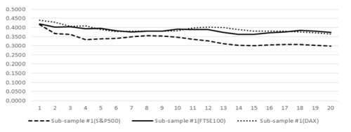
Figure-1. Vol of vol of S&P500, FTSE100 and DAX during sub-sample #1
Note for Figure 1: This figure displays the Vol of vol as a function of k-day for Sub-sample #1of S&P500, FTSE100 and DAX index (Jan 1996 to Dec 2007)
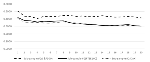
Figure-2. Vol of vol of S&P500, FTSE100 and DAX during sub-sample #2
Note for Figure 2: This figure displays the Vol of vol as a function of k-day for Sub-sample #2of S&P500, FTSE100 and DAX (Jan 2009 to Feb 2016).
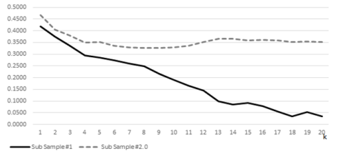
Figure-3. Vol of vol of Sub Sample #1, Sub Sample #2.0 of Nifty Index
Source: Viswanathan and Maheswaran (2016)
Note for Figure 3: This figure displays the Vol of vol as a function of k-day for Sub-sample #1 (Jan 1996 to Dec 2007) and Sub-sample #2.0 (Jan 2009 to April 2015) of Nifty Index. It is borrowed from the paper titled “Back to Normal?” by Lakshmi Viswanathan and S. Maheswaran.
From tables and figures it can be seen, that the long-term stock returns of the three global indices, say S&P500, FTSE100 and DAX, during the pre-crisis as well as the post-crisis period is not normally distributed even for k-day as big as 20. That is to say, there has been no significant change in the structure of volatility of global indices due to the financial crisis of 2008. This finding is strikingly different from the analysis of structure of Vol of vol of Nifty index before and after the crisis, as put forward in the study by Viswanathan and Maheswaran (2016). The study proved that the long-term stock returns of Nifty index, starting from k-day ≥ 10, was normally distributed with constant variance prior to the global financial crisis. However, during the post-crisis period, the Vol of vol remain persistent and does not die down rapidly (Figure 3). Comparing the results of analysis on global indices with Nifty Index, we argue that after the global financial crisis India has joined the league of the developed economies with regard to the structure of volatility.
5. CONCLUSION
In this paper, we have investigated the structure of volatility in stock returns in the global stock markets by analyzing major indices like S&P500, FTSE100 and DAX. We observe that there has been no significant change in the structure of volatility in these indices induced by the global financial crisis of 2008. Vol of vol of long term returns during pre-crisis and post-crisis samples does not die down to zero even for k-day as big as 20. This is in contrast with the case of structure of volatility in Nifty index during pre-crisis period as described by Viswanathan and Maheswaran (2016). There was no evidence of volatility being stochastic in the Nifty index during the pre-crisis period for k-day ≥ 10 which means that long-term returns starting from k-day equal to 10 were approximately normally distributed. However, Vol of vol was found to be positive and persistent during the post-crisis period for Nifty index. This study shows that the structure of volatility of Indian stock market subsequent to the financial crisis of 2008 is similar to the structure of volatility of major global stock markets. In short, evidence suggests that India has joined the big league in terms of the structure of volatility of stock market as a result of the global financial crisis of 2008.
| Funding: This study received no specific financial support. |
| Competing Interests: The authors declare that they have no competing interests. |
| Contributors/Acknowledgement: All authors contributed equally to the conception and design of the study. |
REFERENCES
Baillie, R.T., T. Bollerslev and H.O. Mikkelsen, 1996. Fractionally integrated generalized autoregressive conditional heteroskedasticity. Journal of Econometrics, 74(1): 3-30. View at Google Scholar | View at Publisher
Bollerslev, T., 1986. Generalized autoregressive conditional heteroskedasticity. Journal of Econometrics, 31(3): 307-327. View at Google Scholar | View at Publisher
Bollerslev, T. and H.O. Mikkelsen, 1996. Modeling and pricing long memory in stock market volatility. Journal of Econometrics, 73(1): 151-184. View at Google Scholar | View at Publisher
Breidt, F.J., N. Crato and P. De Lima, 1998. The detection and estimation of long memory in stochastic volatility. Journal of Econometrics, 83(1): 325-348. View at Google Scholar | View at Publisher
Cajueiro, D.O. and B.M. Tabak, 2008. Testing for long-range dependence in world stock markets. Chaos, Solitons & Fractals, 37(3): 918-927. View at Google Scholar | View at Publisher
Cheung, Y.W. and K.S. Lai, 1995. A search for long memory in international stock market returns. Journal of International Money and Finance, 14(4): 597-615. View at Google Scholar | View at Publisher
Clark, P.K., 1973. A subordinated stochastic process model with finite variance for speculative prices. Econometrica: Journal of the Econometric Society, 41(1): 135-155. View at Google Scholar | View at Publisher
Click, R.W. and M.G. Plummer, 2005. Stock market integration in ASEAN after the Asian financial crisis. Journal of Asian Economics, 16(1): 5-28. View at Google Scholar | View at Publisher
Comte, F. and E. Renault, 1998. Long memory in continuous-time stochastic volatility models. Mathematical Finance, 8(4): 291-323. View at Google Scholar | View at Publisher
Di Matteo, T., T. Aste and M.M. Dacorogna, 2005. Long-term memories of developed and emerging markets: Using the scaling analysis to characterize their stage of development. Journal of Banking & Finance, 29(4): 827-851. View at Google Scholar | View at Publisher
Ding, Z. and C.W. Granger, 1996. Modeling volatility persistence of speculative returns: A new approach. Journal of Econometrics, 73(1): 185-215. View at Google Scholar | View at Publisher
Ding, Z., C.W. Granger and R.F. Engle, 1993. A long memory property of stock market returns and a new model. Journal of Empirical Finance, 1(1): 83-106. View at Google Scholar | View at Publisher
Glosten, L.R., R. Jagannathan and D.E. Runkle, 1993. On the relation between the expected value and the volatility of the nominal excess return on stocks. Journal of Finance, 48(5): 1779-1801. View at Google Scholar | View at Publisher
Granero, M.S., J.T. Segovia and J.G. Pérez, 2008. Some comments on Hurst exponent and the long memory processes on capital markets. Physica A: Statistical Mechanics and its Applications, 387(22): 5543-5551. View at Google Scholar | View at Publisher
Granger, C.W. and N. Hyung, 2004. Occasional structural breaks and long memory with an application to the S&P 500 absolute stock returns. Journal of Empirical Finance, 11(3): 399-421. View at Google Scholar | View at Publisher
Granger, C.W. and R. Joyeux, 1980. An introduction to long-memory time series models and fractional differencing. Journal of Time Series Analysis, 1(1): 15-29. View at Google Scholar | View at Publisher
Heyde, C.C. and Y. Yang, 2010. On defining long-range dependence. In selected works of CC Heyde. New York: Springer. pp: 426-431.
Higgins, M.L. and A.K. Bera, 1992. A class of nonlinear ARCH models. International Economic Review, 33(1): 137-158. View at Google Scholar | View at Publisher
Hosking, J.R., 1981. Fractional differencing. Biometrika, 68(1): 165-176. View at Google Scholar | View at Publisher
Hurst, H.E., 1951. {Long-term storage capacity of reservoirs}. Trans. Amer. Soc. Civil Eng, 116: 770-808. View at Google Scholar
Jacobsen, B., 1996. Long term dependence in stock returns. Journal of Empirical Finance, 3(4): 393-417. View at Google Scholar | View at Publisher
Klüppelberg, C., A. Lindner and R. Maller, 2004. A continuous-time GARCH process driven by a Lévy process: Stationarity and second-order behaviour. Journal of Applied Probability, 41(3): 601-622. View at Google Scholar | View at Publisher
Lim, K.P., R.D. Brooks and J.H. Kim, 2008. Financial crisis and stock market efficiency: Empirical evidence from Asian countries. International Review of Financial Analysis, 17(3): 571-591. View at Google Scholar | View at Publisher
Lo, A.W., 1989. Long-term memory in stock market prices (No. w2984). National Bureau of Economic Research.
Lo, A.W. and A.C. MacKinlay, 1988. Stock market prices do not follow random walks: Evidence from a simple specification test. Review of Financial Studies, 1(1): 41-66. View at Google Scholar | View at Publisher
Mandelbrot, B., 1972. Statistical methodology for nonperiodic cycles: From the covariance to R/S analysis. In Annals of Economic and Social Measurement, 1(3): 259-290. View at Google Scholar
Mandelbrot, B.B., 1971. When can price be arbitraged efficiently? A limit to the validity of the random walk and martingale models. Review of Economics and Statistics, 53(3): 225-236. View at Google Scholar | View at Publisher
Mandelbrot, B.B. and N.J.W. Van, 1968. Fractional Brownian motions, fractional noises and applications. SIAM Review, 10(4): 422-437. View at Google Scholar | View at Publisher
Mikosch, T. and C. Starica, 1998. Change of structure in financial time series, long range dependence and the GARCH model. Chalmers Tekniska Högskola/Göteborgs Universitet. Department of Mathematics.
Nelson, D.B., 1990. Stationarity and persistence in the GARCH (l, l) model. Econometric Theory, 6(3): 318-334. View at Google Scholar | View at Publisher
Nelson, D.B., 1991. Conditional heteroskedasticity in asset returns: A new approach. Econometrica: Journal of the Econometric Society, 59(2): 347-370. View at Google Scholar | View at Publisher
Poterba, J.M. and L.H. Summers, 1988. Mean reversion in stock prices: Evidence and implications. Journal of Financial Economics, 22(1): 27-59. View at Google Scholar
Robinson, P.M., 1991. Testing for strong serial correlation and dynamic conditional heteroskedasticity in multiple regression. Journal of Econometrics, 47(1): 67-84. View at Google Scholar | View at Publisher
Robinson, P.M., 2001. The memory of stochastic volatility models. Journal of Econometrics, 101(2): 195-218. View at Google Scholar
Sentana, E., 1995. Quadratic ARCH models. Review of Economic Studies, 62(4): 639-661. View at Google Scholar | View at Publisher
Viswanathan, L. and S. Maheswaran, 2016. Back to normal? Presented at International Conference on Financial Markets and Corporate Finance -2016, Chennai, India.
Zakoian, J.M., 1994. Threshold heteroskedastic models. Journal of Economic Dynamics and Control, 18(5): 931-955. View at Google Scholar | View at Publisher
| Views and opinions expressed in this article are the views and opinions of the author(s), Asian Economic and Financial Review shall not be responsible or answerable for any loss, damage or liability etc. caused in relation to/arising out of the use of the content. |