MATURITIES AND DYNAMIC VOLATILITY OF SUKUK COMPARATIVE STUDY BETWEEN A SUKUK AND A CONVENTIONAL BOND INDEX

Brahim Roukiane¹⁺ --- Abdenbi EL Marzouki²

^1,2Department of Management Sciences Faculty of Legal, Economic and Social Sciences University Mohammed V Agdal Rabat, Morocco

Keywords:Volatility GARCH EGARCH Bond Sukuk Index Maturities.

ARTICLE HISTORY: Received:24 September 2018. Revised:29 October 2018. Accepted:15 November 2018. Published:31 December 2018.

Contribution/ Originality:This article studies the effect of level of maturity on the volatility dynamics of Sukuk indices and conventional bonds, which represents a new research theme. The results of this study can serve both academics and practitioners as a tool for decision support.

1. INTRODUCTION

Over the past decade, several developing countries have begun to focus on issuing Sukuk, as a crucial alternative to conventional bonds to raise funds in the financial market. This increased demand is manifested by the tendency of several Muslim and non-Muslim countries to adopt their regulatory system for issuing Sukuk in their markets. Among these countries are Morocco, Nigeria, South Africa, France, and Kazakhstan, Brunei (Zulkhibri, 2015 ).

The degree of succession and the increased severity of financial crises in recent years have caused excessive volatility, making volatility modeling and forecasting an indispensable element in the financial markets, simply because the concept of volatility has become paramount for many economic and financial applications. For example, portfolio management, risk management and asset valuation.

Volatility is a key indicator that detects fluctuations in the values ​​of an underlying asset or asset class (portfolio or index) around the central trend (Bensafta and Semedo, 2011 ) among the specificities of volatility, Since it is not directly observable, a number of models have been developed that are particularly suitable for estimating the conditional volatility of financial instruments, including the best known and most frequently used models for this volatility. are the autoregressive conditional heteroscedastic models ARCH and GARCH. The main objective of building these models is to make a good forecast of future volatility which will therefore be useful for achieving a more efficient portfolio allocation and risk management (Ahmed, 2011 ).However, some authors show in their research that Sharia-compliant investments (Islamic law) are more financially stable and more profitable, the unique characteristics of the return-risk of Islamic investments have their origins in the respected filtering, which excludes non-compliant enterprises. Sharia  norms (Hakim and Rashidian, 2002 ). It is with this in mind that we have set the objective of comparing the volatility of the Sukuk index with their conventional counterparts. First, we start by comparing the econometric characteristics of each Sukuk index of different maturities with their counterpart. Conventional, using historical volatility measured by the monthly standard deviation, and the conditional volatility estimated by the GARCH and EGARCH models.

We selected a sample of the Sukuk index and conventional bonds of different maturities in the DOW JONES ISLAMIC index family, in daily frequency, over the period from 01/01/2014 to 25/04/2017.

This article will be organized as follows: after a short presentation of our sample and the definition of volatility (section 1), section 2 will cover a brief review of empirical literature. As for Section 3, it will be devoted to the research methodology followed, while Section 4 will deal with the description of the data and the preliminary results. In the end Section 5 will summarize the main results and discussions.

2. CONCEPT OF VOLATILITY

Volatility is an essential tool in the management of financial assets, it combines a set of functions, since it makes it possible to measure uncertainty about the future and refers to the notion of risk, uncertainty about the future price of a financial asset, and finally, it represents a vital indicator on which any investment decision is based.

The importance of this notion has led people to anticipate its variations and changes, since exact anticipation means making the right decision on asset allocation and portfolio management. The techniques for predicting this value based on the assumption of homocedasticity (the variance is constant), they are not fair, because financial assets whose volatility is constant are rare, that's why, Engle (1982 ) proposed the ARCH model, which was generalized (GARCH) by Bollerslev (1986 ).

ARCH / GARCH models consider stock prices as a basis for calculating future volatility. The hypothesis of this method is to benefit from past recorded prices to predict the future.

We then used the ARCH / GARCH models in order to modulate the historical volatilities of the Dow Jones index, in order to compare them with realized volatilities.

In recent years, transactions have increased dramatically in the financial market for Islamic products. It is interesting to model and compare the volatilities of Islamic financial assets with their conventional counterparts, to know if they are really more resistant to crises than conventional assets.

Volatility has several characteristics that make speculation attractive:

• It increases when the risk increases.
• It returns to medium (high volatilities will likely decrease and low volatilities will likely increase).

Then, volatility is often negatively correlated with the price of the asset where the level of the index.

3. LITERATURE REVIEW

As far as academic research is concerned, Islamic index do not consider themselves as a research subject, as they have a recent history and are also related to certain methodological problems due to differences due to size and sector weighting (Fowler and Hope, 2007 ). Indeed, the number of academic works on volatility and the causal link between Islamic clues or between Islamic and conventional clues remains limited. Thus, Rahim et al. (2009 )  examines the transmission of volatility as well as the correlation between the Kuala Lumpur Syariah index and the Islamic index of Jakarta. The duration of their study runs from July 4 to December 29, 2006. In practice, the authors generally use the GJR-GARCH model, which captures the correlation between profitability and future volatility. The authors show that there is a transmission of the volatility of the Islamic stock market, from Malaysia to the Indonesian Islamic stock market, but, conversely, they find no significant transmission of the Indonesian market to the Malaysian market, which translates an asymmetrical transmission. In reality, it seems that a unidirectional flow of information between the two markets is observed. Finally, they find a weak correlation between the two markets. Moreover, the causal examination between the Islamic stock market and their conventional counterparts, a particular interest is given to the examination of volatility.

However, other studies look at the Sukuk market as that of Cakir and Raei (2007 ) they studied the differences between Sukuk and Eurobonds, and they modeled the impact of bonds issued according to Islamic norms (Sukuk), on the cost and the nature of the investment portfolio risks. Using the Value-t-Risk (VAR), the delta-normal and Monte-Carlo simulation methods, they found that according to different price behaviors, Sukuk are totally different instruments compared to conventional bonds. In the same context (Fathurahman and Fitriati, 2013 ) compare Sukuk returns and conventional bonds through the comparison of risk, return and correlation variables. They conclude that the average yield of Sukuk is greater than the average yield of conventional bonds. In terms of risk, the Sukuk standard deviation is relatively larger than the standard deviation of conventional bonds. In the risk management section (Shafi and Ariffin, 2013 ) find strategies to reduce the risk of Sukuk, through their proposal for a model of Sukuk with integrated option and a mathematical model for the valuation of returns before conversion. They proposed the use of Sukuk with built-in options to mitigate Sukuk risk. The built-in options are a way to mitigate the risk, so the study proposes to use real assets like real estate assets.

While, the study by Nafis et al. (2013 ) examines the impact of Sukuk and the announcement of conventional bonds and wealth of shareholders. Using 79 Sukuk and 87 conventional bonds over the period 2004-2012 in the financial markets of six developed Islamic countries. The study shows that in a short-term perspective, the effect of the Sukuk announcement on the negative enterprise value, while the effect of the announcement of the conventional bond is positive for all periods except the post-crisis period. Therefore, apart from the religious motivation on the Sukuk show, the negative effect could prevent companies from raising funds for the Sukuk.

In another article, conduct comparative studies between Islamic index and their conventional counterparts, but in the stock market such as that of  Kassab (2013 ) he empirically explores the persistence of the volatility of the Islamic stock market index (DJIM) and the 'conventional stock index (S & P 500 index) over a period from December 29, 2006 to March 07, 2011. Using the GARCH model, he finds that the persistence of the volatility of the two types of index is very significant. They also show that the Islamic index S & P500-shariah is actually less volatile than its conventional S & P500 consortium, and that it has a low risk during the crisis period (Yusof and Majid, 2007 ) examine whether conditional volatility in Malaysia's conventional and Islamic stock markets is sensitive to US interest rate volatility. Considering the period from January 1992 to December 2000, using the GARCH-M models (a model where the conditional variance is an explanatory variable of the conditional mean), GARCH (1,1) and the VAR model, their results indicate that interest rate volatility affects stock market volatility conventional but not the Islamic stock market, which implies that the stabilization of the interest rate would not affect the volatility of the stock market Islamic.

In terms of portfolio diversification advantage combining Islamic assets and conventional, Akhtar et al. (2011 ) conducted a comparative study on volatility between different combinations of Islamic and conventional banking assets. They show that the introduction of an Islamic banking asset into a portfolio, by controlling the specific characteristics of each asset in each country, can reduce the volatility intensity by 7.17 points.

More recently, Chau et al. (2013 ) examine the effect of political uncertainty (caused by the civil insurrections of the "Arab Spring" on the volatility of stock markets in the MENA region (Bahrain, Lebanon, Kuwait, Oman, Jordan and Egypt) over a period from June 1, 2009 to June 29, 2012. By distinguishing the Islamic stock market indexes from the conventional stock market index, the authors show that the two types of investments react in heterogeneous ways to recent political unrest. More specifically, the results show a significant increase in the volatility of Islamic index during the period of political dissent. While the volatility of conventional stock index has not been infected by political uncertainty. This difference is confirmed by a complementary analysis of the multi-variate GARCH model. By examining the causal link between the Islamic stock market and the stock market conventional methods, Ajmi et al. (2013 ) highlight a linear causal relationship and non-linear between these two markets, they found that there is a strong c relationship between the Islamic stock market and other stock markets (Kim and Kang, 2012 ) analyze the mechanism of the transmission of volatility between Islamic stock market and the bond market in Malaysia. By adopting a modeling of the type VAR-bivariate-GARCH and VECM-bivariate GARCH, the results show that there is a transmission of unidirectional volatility from the Islamic stock market to the bond market during the crisis period, which implies that the stock market Islamic has a strong influence on the Sukuk market. The analyzes also indicate that there is no transmission of volatility from the bond market to the Islamic stock market. Chiadmi and Ghaiti (2012 ) study the persistence of the volatility of the Islamic index S & P500-Shariah and its conventional counterpart S & P-500 over a period of 11 from December 2006 to March 07, 2011. The results of the GARCH model show that the persistence of the volatility of the two types of index is very significant and that the index S & P500-Sharia is less volatile and low risk during a time of crisis compared to its conventional counterpart.

4. DATA AND METHODOLOGY

4.1. The data

The objective of this study is to analyze the dynamics of volatility between Sukuk and conventional bonds, as well as to examine the causal link between the two types of assets. In this context, we have created a sample of ten Sukuk stock index in the DOW JONES index family, for ease of comparison we have chosen five Sukuk index of different maturities and their conventional counterpart (Table 1). In the BLOOMBERG database we have selected the daily closing price data covering the study period 02/01/2014 - 25/04/2017. The choice of our sample is motivated by the availability of statistical data and the difficulty accessing databases that provide a wide range of index types.

Table-1. Sukuk index and their conventional counterpart

Sukuk Index1		Conventional Bonds Index2
Index	Bloomberg	Index	Bloomberg
Dow Jones Sukuk 1 -3 Year Total Return Index	DJSUK3T	S&P 0-3 Year High Yield Corporate Bond Index	SPUSHY3T
Dow Jones Sukuk 3 -5 Year Total Return Index	DJSUK5T	S&P 3-5 Year High Yield Corporate Bond Index	SPUSHY5T
Dow Jones Sukuk 5 – 7 Year Total Return Index	DJSUK7T	S&P 5-7 Year High Yield Corporate Bond Index	SPUSHY7T
Dow Jones Sukuk 7-10  Year Total Return Index	DJSUK10T	S&P 7-10 Year High Yield Corporate Bond Index	SPUSHY10T
Dow Jones Sukuk Index	DJSUKUK	S&P U.S. Issued High Yield Corporate Bond Index	SPUSCHY

Source: S&P Dow Jones Indices.

After collecting the historical data of the index of our sample we calculated the logarithmic daily yields, in order to mitigate the heteroscedasticity and to keep the additivity of the financial series. The daily yields R_t are calculated by the following formula:

With Pt is the closing index price at the date t.

In order to compare the series of the returns of the Sukuk index and their conventional counterpart, we called the Student test (t-test) which made it possible to test the following hypotheses: H0: the averages of the returns of the two index are equal, against the alternative hypothesis H1: the averages of the returns of the two index are deferential.

4.2. Granger Causality Test

In econometrics, the concept of causality introduced by Granger (1969 ) is based on the search for links of dependencies between two financial series. Indeed, a variable Y "causes according to Granger" and a variable X if the parameters of the past values of the variable Y are significantly different from zero. In a more general way, we can write the following equation representing the starting point of the test:

Y said the Granger X sense, if the parameters y_t of the past values of X are significantly different from zero.

In our study we used Granger causality tests to detect causal links between Sukuk index returns and their conventional counterparts. We have tried to apply these Granger tests to model the bidirectional and unidirectional causal links between the Sukuk index and their conventional counterparts.

4.3. Volatility Measures

Volatility is an indispensable statistical tool in the financial market which makes it possible to measure the risk of the variability of the yields of the index returns. Indeed volatility is a measure to study the dispersion of returns of financial assets around their average return. In our study we used two types of volatilities, namely: historical volatility also called unconditional volatility and conditional volatility based on GARCH models.

4.4. Unconditional Volatility

As a first step we have calculated the historical (unconditional) volatility using the unbiased standard deviation of the rate of return changes, it is estimated ex-post on the basis of past returns. The estimated standard deviation of daily returns can be used as a tool to measure volatility, as it measures the dispersion of returns on the mean by the following formula.

If the standard deviation is large, means that there is a high probability of capturing a high yield in the positive or negative direction, it is worth saying that the volatility of the returns is high.

4.5. Conditional Volatility

4.5.1. The GARCH Model

This part will be devoted to modeling the conditional volatility of the returns of the index of our sample, using the models of the GARCH family, which were introduced by Bollerslev (1986 ). Indeed, these models allowed us to make an autoregressive representation of the conditional variance of the series of returns of our index. In this context, the conditional variance of each series of returns is estimated by the square of the p past error terms and the delayed conditional variances. Thus, the conditional variance is calculated by the following formula:

With βj represents the autoregressive coefficient which gives an explanation of the impact of past volatilities on current volatility, ie. the impact of shocks on performance.

Asymmetry is a central property for the study of financial series, but ARCH and GARCH type models do not take this hypothesis into account, which leads us to use the EGARCH model.

4.5.2. The EGARCH Model

The models of GARCH are characterized by the estimate of the residues squared, which hides the impact of the bearish or bullish movements, the models of EGARCH introduced by Nelson (1991 ) aim at making up for this insufficiency, they make it possible to model the influence of the bearish and bullish movements on the behavior of financial series. This model may be represented as follows:

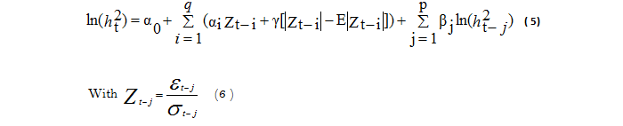
which represent the standardized error, based on the remark empirically that the volatility of financial assets tends to increase after peaks of negative returns, in contrast to peaks of positive returns. This finding has been taken into account in the EGARCH model by taking into consideration the signs of past residues in the calculation of the conditional variance. On the other hand, the GARCH model, the EGARCH model, assumes no assumptions about the parameters to ensure the positivity of the conditional variance. The presence of negative and positive values ​​in the equation allowed different impacts on volatility. Having a negative coefficient means a negative yield shock that generates higher volatility than a positive shock. Indeed, the main difference between the GARCH model and EGARCH lies in the fact that the latter takes into account that bad news has different impacts compared to good news on volatility.

5. RESULTS AND DISCUSSIONS

5.1. Descriptive Statistics

Analyzing the returns distributions of the index is a crucial step to get an idea of the behavior of the series of daily returns of the index of our sample.

Table-2. The characteristics of the series of returns

	Pair 1		Pair 2		Pair 3		Pair 4		Pair 5
Indice	SPUSHY10T	DJSUK10T	SPUSHY7T	DJSUK7T	SPUSHY5T	DJSUK5T	SPUSHY3T	DJSUK3T	SPUSCHY	DJSUKUK
Mean	0.000232	0.000089	0.000199	0.000141	0.000174	0.000243	0.000208	0.000252	0.000208	0.00002.
Median	0.000469	0.000125	0.000311	0.000143	0.000292	0.000275	0.00026	0.000281	0.000359	0.000096
Maximum	0.014896	0.003267	0.01377	0.003633	0.008993	0.013292	0.005961	0.009909	0.011331	0.004202
Minimum	-0.01404	-0.00398	-0.01431	-0.0049	-0.01179	-0.01275	-0.00638	-0.02483	-0.01369	-0.01029
Std. Dev.	0.003087	0.000494	0.002786	0.000782	0.002209	0.002241	0.001164	0.002276	0.002477	0.001092
Skewness	-0.41303	-1.02845	-0.50167	-0.56684	-0.88209	0.025784	-1.08014	-1.9509	-0.62441	-1.59143
Kurtosis	7.053791	13.11963	7.648255	7.441754	8.197218	8.25967	9.614343	25.80466	8.000671	17.92153
Jarque-Bera	591.2007	3683.446	781.0888	725.873	1040.513	953.3514	1672.38	18489.35	917.6423	8040.705
Probability	0	0	0	0	0	0	0	0	0	0

Source: EViews 7

Table 2 presents the main descriptive properties of the series of returns of the Sukuk index and their conventional counterparts (mean, median, maximum, minimum, standard deviation, Skewness, kurtosis and Jarque Bera test).

We find that the averages of the returns of the index in our sample are all positive as well as the average yields of the Sukuk index are higher than their conventional counterparts if the maturity is less than 5 years and vice versa if the maturity exceeds 5 years. Looking at the standard deviation we can easily notice that if the maturity is less than 5 years, the standard deviation of the Sukuk yield series is greater than the standard deviation of their conventional counterpart, and the opposite if the maturity is greater than 5 years.

The SKEWNESS coefficients of the index are all negative, except that of the DJSUK5T index which is positive, which means that the distributions of the series of the returns of the index are asymmetrical, the downward movements are stronger than the upward movements. Examining the KURTOSIS coefficients, we find that the distributions of the series of the returns of all the index have long distribution tails, since the coefficient is much greater than 3, which means that the tails are thicker on the ends than those of the normal law, this result allows us to assume the presence of a non-linear (dynamic) distribution, because in general, volatility depends on the past.

The Jarque-Bera test in Table 2 rejects the normality assumption of the distributions of all series of index returns in our sample. These statistical properties confirm the classic features of financial series, including negative asymmetry and thick distribution tails.

In the graphs that follow (Figure 1) we represent the series of returns of the stock index of Sukuk of different maturities and their conventional counterparts. The visual examination of the graphs shows that the returns of the Sukuk index are all less volatile than those of conventional bonds. We can also notice that generally the returns of the Sukuk index and the conventional bond index, they do not have the same downtrend that it is or bullish. This allows us to assume the lack of causality between each index and its counterpart.

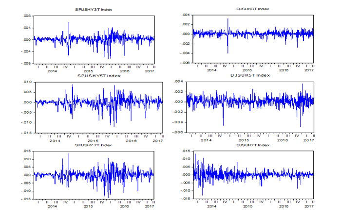
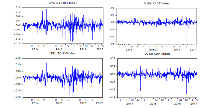
Figure-1. Evolution of the returns of the index of the Sukuk of different maturity and their conventional counterparts

Source: EViews 7

Generally we notice the presence of periods of high volatility in the market (the volatility group), this behavior can not be taken into account using ARMA models, we also note that the series of returns has trajectories compatible with second-order stationarity.

5.2. Student's Test

We perform the Student test to see whether the calculated differences between the Sukuk index and their cohorts are statistically significant. Indeed, the application of this test requires the normality of the distribution, against the absence of the latter can skew the results. In our sample, we calculated daily data for these index over three years, which allows us to construct financial series of 830 observations. Since the size of our sample is greater than 30, we can assume that the distributions of our series are all following a normal distribution.

Table-3. Average Comparison Test

Index		Mean	Standard deviation	T-Student	sig
Pair 1	SPUSHY3T Index - DJSUK3T Index	,00011784	,00112319	3,021	,003
Pair 2	SPUSHY5T Index - DJSUK5T Index	,00003295	,00215091	,441	,659
Pair 3	SPUSHY7T Index - DJSUK7T Index	-,0000431	,0032496	-,382	,703
Pair 4	SPUSHY10T Index - DJSUK10T Index	-,0000209	,0028531	-,211	,833
Pair 5	SPUSCHY Index - DJSUK10T Index	-,0000444	,0025452	-,502	,616

Source: EViews 7

The results presented in Table 3 show that generally the differences in the returns of the index studied are not statistically significant, with the exception of the returns of maturity index less than 3 years, which gave a significant Student test. This means that the series of DJSUK3T and SPUSHY3T yields are significantly different on average (Sig = 0.003). In conclusion, the test of Student of equality of the averages, allows to conclude that there is no difference between the index of Sukuk and their consorts conventional except for the index of maturity of less than 3 years.

5.3. Causality in the Sense of Granger

To detect the possible links between the Sukuk index and their conventional counterparts, we calculate the Granger causality test. It makes it possible to compare and visualize the returns of each Sukuk index and its conventional counterpart. However, they provide very relevant information regarding the meaning of the transmission of information.

Table-4. Summary of Granger causality tests

Null Hypothesis:	F-Statistic	Prob.
DJSUKUK_INDEX does not Granger Cause SPUSCHY_INDEX	1.15838	0.314506
SPUSCHY_INDEX does not Granger Cause DJSUKUK_INDEX	15.44481	2.60E-07***
DJSUK10T_INDEX does not Granger Cause SPUSHY10T_INDEX	2.393058	0.091986
SPUSHY10T_INDEX does not Granger Cause DJSUK10T_INDEX	21.77266	6.11E-10***
DJSUK3T_INDEX does not Granger Cause SPUSHY3T_INDEX	0.373212	0.688636
SPUSHY3T_INDEX does not Granger Cause DJSUK3T_INDEX	5.724856	0.00339534***
DJSUK5T_INDEX does not Granger Cause SPUSHY5T_INDEX	0.057623	0.94401
SPUSHY5T_INDEX does not Granger Cause DJSUK5T_INDEX	6.387136	0.001767808***
DJSUK7T_INDEX does not Granger Cause SPUSHY7T_INDEX	0.882531	0.414126
SPUSHY7T_INDEX does not Granger Cause DJSUK7T_INDEX	3.297395	0.037469134**

**, *** significance at thresholds of 5%, 1% respectively

Source: EViews 7

Analyzing Table 4, we note the presence of unidirectional relations between the returns of Sukuk index of all maturities and their conventional consorts. Indeed, these causal relations are all in the same direction, according to which the returns of the index of the conventional bonds cause significantly in the sense of Granger the returns of the index of the Sukuk. In other words, the returns of conventional bond index can contribute to the prediction of that of the Sukuk index.

5.4. Unconditional Volatility

In order to model the dynamics of the volatility of the Sukuk index and their conventional counterparts, we have calculated the historical historical volatility of each index. Indeed, we calculate the monthly standard deviation of each performance index. The graphs in Figure 2 describe the dynamics of monthly unconditional volatility (the standard deviation) of the returns of the Sukuk index of different maturities and their conventional counterparts.

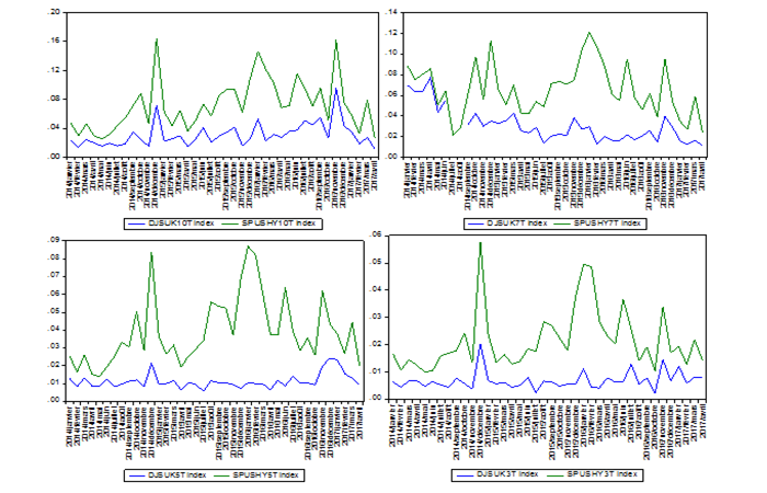
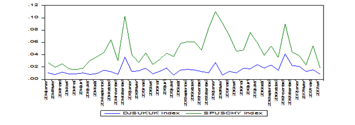
Figure-2. Monthly unconditional volatility (standard deviation) of Sukuk index of different maturities and their conventional counterparts.

Source: EViews 7

From the graphs in Figure 2, we note that the Sukuk index are all less volatile than the conventional bond index, we can also note that the historical volatilities of each index and their counterparts behave in the same way. Indeed, the peaks of volatility occur on the same dates, but with different magnitudes, these corresponding to the financial shocks.

5.5. Conditional Volatility

5.5.1. GARCH Models

After studying the econometric characteristics of each series of index returns. We will perform heteroscedasticity tests to detect the importance of applying ARCH and GARCH models.

Table-5. Ljung-Box Test

Indice	Ljung-Box-Q(1)
SPUSHY10T	283.43	0
DJSUK10T	346.31	0
SPUSHY7T	275.09	0
DJSUK7T	372.23	0
SPUSHY5T	292.12	0
DJSUK5T	361.8	0
SPUSHY3T	285.67	0
DJSUK3T	363.95	0
SPUSCHY	282.31	0
DJSUKUK	307.8	0

Source: EViews 7

The Ljung and Box (1978 ) test that we performed on all the index in our sample allowed us to notice that the correlations are all significant, since the gains associated with the LJUNG-BOX statistics are all less than 5%. We therefore conclude the rejection of the hypothesis of homoscedasticity of series of returns of all index. Indeed, there is an ARCH effect for all indexes the returns of our sample.

These results led us to model conditional volatility by performing the famous GARCH model (1.1). The minimization of the AKAIKE criteria has proposed us to use the Gaussian distribution with respect to the Student distribution and the GED distribution.

Table-6. Summarizes the results of the GARCH model estimates (1,1).

	Indice		c	α	β	α + β
Maturity between 7 years and 10 years	SPUSHY10T		3.01E-07***	0.531201***	0.562151***	1.09335
		z-Statistic	4.660822	11.08616	23.63805
	DJSUK10T		4.91E-07***	0.377262***	0.614979***	0.992241
		z-Statistic	6.675731	15.70964	30.36823
Maturity between 5 years and 7 years	SPUSHY7T		1.52E-07***	0.406165***	0.652903***	1.059068
		z-Statistic	4.836286	10.87092	31.03929
	DJSUK7T		3.34E-08***	0.045141***	0.94297***	0.988111
		z-Statistic	3.434003	6.340855	122.5746
Maturity between 3 years and 5years	SPUSHY5T		1.25E-07***	0.491358***	0.584165***	1.075523
		z-Statistic	4.586664	10.9064	24.14609
	DJSUK5T		1.41E-07***	0.203175***	0.569734***	0.772909
		z-Statistic	4.931483	7.771866	9.155699
Maturity between 1 years and 3years	SPUSHY3T		5.01E-08***	0.30876***	0.686973***	0.995733
		z-Statistic	5.386517	8.094973	24.45502
	DJSUK3T		4.58E-08***	0.21134***	0.587955***	0.799295
		z-Statistic	5.593024	7.91902	11.66811
Market index	SPUSCHY		1.76E-07***	0.495338***	0.580738***	1.076076
(all maturities)		z-Statistic	5.439613	10.50368	22.04167
	DJSUKUK		2.08E-07***	0.37385***	0.513174***	0.887024
		z-Statistic	6.084155	11.01833	12.38181

*** Significance at the 1% threshold

Source: EViews 7

After the first reading of Table 6, we find that all the coefficients of the GARCH model (1,1) are positive and are all significant at the 1% threshold for all index in our sample. This finding allows us to conclude that the GARCH model (1,1) has successfully modeled the behavior of index returns in our sample. We can note as easily as the coefficients α of the equation of the model GARCH (1,1) are all lower than the values ​​of the coefficients β. This is a sign that the market is causing significant corrections in future conditional volatility and also that the conditional variance is certainly impacted by past variance, implying that past information shocks have a significant impact on current returns. . The first parameter c means the threshold of the minimum conditional variance, we notice that it is almost negligible (close to 0) for all the index of our sample. The second parameter α is a coefficient that captures the impact of shocks on volatility, it is calculated by summing the residuals to the squares, in Table 6, we note that the coefficient of the Sukuk index is much lower than that of the bonds conventional.

The third parameter β aims to measure the persistence of the volatility, it is obtained by the sum of the delayed variances. Indeed, it gives an idea of ​​the contribution of past volatilities in current volatility. We can easily notice in Table 6 that if the maturity is less than 5 years the coefficient β of the Sukuk index is slightly lower compared to its conventional counterpart, and the opposite if the maturity is greater than 5 years. This means that the persistence of the volatility of the Sukuk index is more persistent compared to its conventional counterpart if the maturity exceeds strictly 5 years and vice versa if the maturity is less than 5 years.

The sum of the parameters α + β for all the index of the yields are lower than 1 for all Sukuk index, which implies the stationarity of the conditional volatility of these index. For conventional bond index, this sum is greater than 1 for all maturities except for maturity between 1 year and 3 years. Indeed, the calculation of the coefficients (α + β) gives important information on the extent of the persistence of the conditional volatility.

In this section we applied the GARCH model (1,1) for all series of index returns of our sample, we graphically represented the conditional volatility of our series in graph 3.

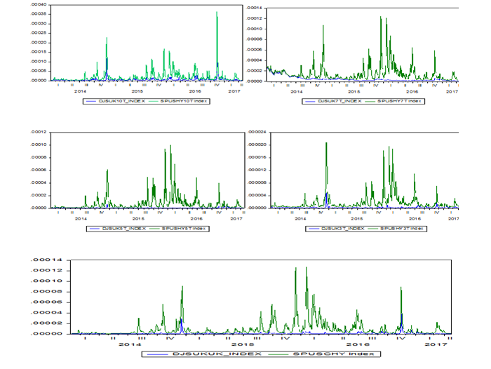
Figures-3. Evolution of conditional volatility estimated by GARCH models (1,1)

Source: EViews 7

Given the above figures, which represent the dynamics of the volatility of index returns, we generally observe that volatility peaks occur on the same dates, however, with widely differing degrees, indicating that the degree of impact is Financial shocks on the Sukuk index are totally different to this one on conventional bonds. It is also clear from the graphs that all Sukuk index are significantly and significantly less volatile than their conventional counterparts, which allows us to conclude that the Sukuk index are more stable than their counterparts.

5.5.2. EGARCH Models

In order to deepen our modeling, we have integrated the phenomenon of asymmetry for the behavior of volatility. The EGARCH models introduced by Nelson (1991 ) are used to analyze the asymmetry of conditional volatility. Table 7 presents the results of different model estimates EGARCH (1,1).

Table-7. EGARCH Model Parameters (1.1)

Indice		C	α	Γ	β
SPUSHY10T		-1.304913***	0.489232***	-0.177766***	0.923778***
	z-Statistic	-9.11176	9.07412	-6.98893	86.09271
DJSUK10T		-1.895150***	0.485120***	-0.153801***	0.875285***
	z-Statistic	-9.35438	17.08502	-7.64879	53.51906
SPUSHY7T		-0.946134***	0.417706***	-0.136162***	0.949835***
	z-Statistic	-8.61995	10.00857	-6.82091	119.5389
DJSUK7T		-0.220214***	0.137556***	-0.043128***	0.990803***
	z-Statistic	-5.60192	7.157209	-4.51152	346.7359
SPUSHY5T		-1.234556***	0.526592***	-0.134474***	0.935854***
	z-Statistic	-8.36473	11.59804	-6.03548	87.65435
DJSUK5T		-0.690748***	0.151648***	-0.056021***	0.959192***
	z-Statistic	-4.03068	5.778717	-4.56755	86.73075
SPUSHY3T		-1.032696***	0.358349***	-0.113332***	0.945962***
	z-Statistic	-7.03033	8.945425	-6.66961	101.3005
DJSUK3T		-2.607324***	0.273976***	-0.192236***	0.844761***
	z-Statistic	-6.15752	7.299221	-7.98469	31.81736
SPUSCHY		-1.265303***	0.500364***	-0.146113***	0.930581***
	z-Statistic	-8.86163	9.860302	-6.18594	92.51607
DJSUKUK		-2.805448***	0.500543***	-0.125537***	0.823849***
	z-Statistic	-8.1374	14.51136	-5.64856	33.67699

*** Significance differ from zero to 1%

Source: EViews 7

From Table 7, we note that all coefficients of the EGARCH (1,1) model are significant, which implies the presence of the asymmetry effect for all index in our sample. This remark implies that the impact of negative returns on volatility is greater than the impact of positive returns. By examining the α parameters that measure the impact of financial shocks on returns, we find that the degree of impact of financial shocks is lower for Sukuk index than for their conventional counterparts. Regarding the γ coefficients, we notice that they are all negative and significant at 1%, it is a sign of the presence of the effect of the lever, which implies that the index of our sample are more sensitive to the bad news (Bad news) and good news. This remark allows us to conclude that negative financial shocks have a stronger impact on volatility than positive shocks for all index in our sample. The β coefficients are used to calculate the magnitude of the impact of past volatility on current volatility, ie the presence of volatility groups (volatility cluster), because all the β coefficients are positive and significant for all the index. Sukuk and their consorts. Note also that we are in the presence of stationary series, as all the coefficients β are less than 1.

In order to visualize the behavior of the conditional volatility obtained by estimating the EGARCH (1,1) models, Figures 4 present the dynamics of the volatility of each Sukuk performance index and their conventional consorts.

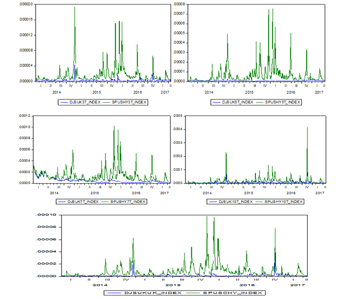
Figures-4. Evolution of the conditional volatility estimated by the EGARCH model (1,1)

Source: EViews 7

From Figure 3, we can definitely conclude from the graphs that all Sukuk index are largely and significantly less volatile than their conventional counterparts, which reinforces the results obtained by applying GARCH models (1,1).

6. CONCLUSION

Throughout this article, we have tried to compare the dynamics of the volatility of Sukuk index of different maturities and their conventional counterparts by performing several tests, namely the Student test, the Granger causality test, the test. of Jarque Berra and the test of Ljung-Box e ARCH. Thus we modeled the behavior of volatility using the unconditional volatility measured by the standard deviation and the conditional volatility estimated by the models GARCH (1,1) and EGARCH (1,1).

The results of Student's tests show that there is no significant difference between the average returns of the two index, except for maturity index of less than 3 years. For the Granger causality test, we note that there is a unidirectional causal relationship in each index pair. Indeed the returns of conventional bonds of different maturities cause in the sense of Granger their consort of Sukuk. In calculating the unconditional volatility estimated by the monthly standard deviation we find that the Sukuk index have the same behavior as their conventional counterparts but with widely different magnitudes. Indeed, Sukuk index are much less volatile than index of conventional bonds of the same maturity.

The modeling of the volatility of the returns index by the GARCH and EGARCH models shows that the Sukuk index are significantly and largely less volatile than their conventional counterparts for all maturities, as well as the volatility of the Sukuk index is more persistent compared to their conventional counterparts if the maturity exceeds strictly 5 years and vice versa when the maturity is less than 5 years.

Finally, we conclude that Sukuk are generally less risky than conventional bonds because of the fact that in a conventional bond the relationship between the subscriber and the issuer is identical to that of a debtor and a creditor. Sukuk is generally a part of property in real and tangible assets, which minimizes the degree of taxation at various risks.

Funding: This study received no specific financial support.

Competing Interests: The authors declare that they have no competing interests.

Contributors/Acknowledgement: Both authors contributed equally to the conception and design of the study.

REFERENCES

Ahmed, A.E.M., 2011. Modeling stock market volatility using GARCH models evidence from Sudan. International Journal of Business and Social Science, 2(23).

Ajmi, A.N., S. Hammoudeh, D.K. Nguyen and S. Sarafrazi, 2013. How strong are the causal relationships between islamic stock markets and conventional financial systems? Evidence from linear and nonlinear tests. Journal of International Financial Markets, Institutions and Money, 28(C): 213-227.

Akhtar, S., M. Jahromi, K. John and C. Moise, 2011. Intensity of volatility linkages in islamic and conventional markets. 24th Australasian Finance and Banking Conference 2011 Paper.

Bensafta, K.M. and G. Semedo, 2011. Shocks, shocks of volatility and contagion between. Economic Review, 62(2): 277-311.

Bollerslev, T., 1986. Generalized autoregressive conditionnal heteroscedasticity. Journal of Economic Surveys, 31(3): 307-327. Available at: https://doi.org/10.1016/0304-4076(86)90063-1.

Cakir, S. and F. Raei, 2007. Sukuk vs. Eurobonds: Is there a difference in value-at-risk?« IMF Working Paper, No WP/07/237. Wachington, DC: International Monetary Fund.

Chau, F., R. Deesomsak and J. Wang, 2013. Political uncertainty and stock market volatility in the Middle East and North African (MENA) countries. Journal of International Financial Markets, Institutions and Money, 28(C): 1-19. Available at: https://doi.org/10.1016/j.intfin.2013.10.008.

Chiadmi, M. and F. Ghaiti, 2012. Modeling volatility stock market using the ARCH and GARCH models: Comparative study between an Islamic and a conventional index (SP Sharia VS SP 500). International Research Journal of Finance and Economics, 91: 138-146.

Engle, R.F., 1982. Autoregressive conditional heteroscedasticity wed estimates of the variance of U.K inflation. Econométrica, 50(4): 987-1008. Available at: https://doi.org/10.2307/1912773.

Fathurahman, H. and R. Fitriati, 2013. Comparative analysis of return on sukuk and conventional bonds. American Journal of Economics, 3(3): 159-163.

Fowler, S.J. and C. Hope, 2007. A critical review of sustainable business index and their impact. Journal of Business Ethics, 76(3): 243–252. Available at: https://doi.org/10.1007/s10551-007-9590-2.

Granger, C.W., 1969. Investigating causal relations by econometric models and cross-spectral methods. Econometrica, 37(3): 424-438. Available at: https://doi.org/10.2307/1912791.

Hakim, S. and M. Rashidian, 2002. Risk and return of Islamic stock market indexes. 9th Economic Research Forum Annual Conference in Sharjah, UAE. pp: 26-28.

Kassab, S., 2013. Modeling volatility stock market using the ARCH and GARCH models: Comparative study index (SP Sharia VS SP 500). European Journal of Banking and Finance, 10: 72-77.

Kim, H.B. and S.H. Kang, 2012. Volatility transmission between the Sharia stock and sukuk GII markets in Malaysia. Available from https://search.yahoo.com/search;_ylt=AuynaOiNRkSG9bf6F4qvcFebvZx4?p=volatility%2C+causality+and+Islamic+markets&toggle=1&cop=mss&ei=UTF-8&fr=yfp-t-900.

Ljung, G.M. and G.E. Box, 1978. On a measure of lack of fit in time series models. Biometrika, 65(2): 297-303. Available at: https://doi.org/10.2307/2335207.

Nafis, A., M.K. Hassan and M.A. Haque, 2013. Are islamic bonds different from conventional bonds? International evidence from capital market tests. Borsa Istanbul Review, 13(3): 22-29. Available at: https://doi.org/10.1016/j.bir.2013.10.006.

Nelson, D.B., 1991. Conditional heteroskedasticity in asset returns: A new approach. Econometrica, 59(2): 347-370. Available at: https://doi.org/10.2307/2938260.

Rahim, A.F., N. Ahmad and I. Ahmad, 2009. Information transmission between Islamic stock indices in South East Asia. International Journal of Islamic and Middle Eastern Finance and Management, 2(1): 7-19. Available at: https://doi.org/10.1108/17538390910946230.

Shafi, R.M. and N.A. Ariffin, 2013. Sukuk structure with embedded options as risk mitigation tool. Paper Presented at the Minth Internationnal Conference of Islamic Econmics and Finance, Istanbul, Turkey.

Yusof, M.R. and A. Majid, 2007. Stock market volatility transmission in malaysia: Islamic versus conventional stock market. Journal of King Abdulaziz University: Islamic Economics, 20(2): 19-40. Available at: https://doi.org/10.4197/islec.20-2.2.

Zulkhibri, M., 2015. A synthesis of theoretical and empirical research on sukuk. Borsa Istanbul Review, 15(4): 237-248. Available at: https://doi.org/10.1016/j.bir.2015.10.001.

---