


HIDDEN MARKOV MODEL FOR TIME SERIES PREDICTION

1Department of Mathematics & Statistics, ARID Agriculture University Rawalpindi, Pakistan
2,4Department of Statistics, University of Sargodha, Pakistan
3Punjab Agriculture Department, Sargodha, Pakistan
ABSTRACT
The Hidden Markov Model (HMM) is a powerful statistical tool for modeling generative sequences that can be characterized by an underlying process generating an observable sequence. Hidden Markov Model is one of the most basic and extensively used statistical tools for modeling the discrete time series. In this paper using transition probabilities and emission probabilities different algorithm are computed and modeled the series and the algorithms to solve the problems related to the hidden markov model are presented. Hidden markov models face some problems like learning about the model, evaluation process and estimate of parameters included in the model. The solution to these problems as forward-backward, Viterbi, and Baum Welch algorithm are discussed respectively and also useful for computation. A new hidden markov model is developed and estimates its parameters and also discussed the state space model.
© 2017 AESS Publications. All Rights Reserved.
Keywords: Hidden markov model Estimators, Time series, Algorithm, States, Sequence, Probability.
Article History: Received: 17 February 2017, Revised: 4 April 2017, Accepted: 10 May 2017, Published: 15 June 2017
1. INTRODUCTION
The Hidden Markov Model (HMM) is a powerful statistical tool for modeling generative sequences that can be characterized by an underlying process generating an observable sequence. HMMs have found application in many areas interested in signal processing and particularly in speech processing. Hidden Markov Model is one of the most basic and extensively used statistical tools for modeling the discrete time series.
A Hidden markov model is a limited learnable stochastic device. It is the summation of stochastic process having the following two aspects. Firstly, stochastic process is a limited set of states, so that every state is connected with multidimensional probability distribution function. The transitions among the different states are located as a set of probabilities known as transition probabilities. Secondly in stochastic process, the states are ‘hidden’ to the observer are to be observed on its occurrence. So that it is named as “hidden markov model”. The states, symbols, transition probabilities, emission probabilities and initial probabilities joined together to form a hidden markov model.
Time series data have a natural chronological order. So time series analysis differs from cross-sectional study, in which there is no natural ordering of the observations. Time series analysis is also dissimilar from spatial data analysis where the observations usually relate to geographical locations (e.g. accounting for house prices by the location as well as the inherent characteristics of the houses). A stochastic model for a time series will generally return the fact that observations close together in time will be more closely related than observations further apart. Time series analysis can be applied to real-valued, continuous data, discrete numeric data, or discrete symbolic data.
Prediction can be done when the model is in the form of transferred function or in terms of state space parameters, smoothed and filtered. If the model is linear than a minimum-variance Kalman filter and minimum variance smoothers are used. Prediction of chaotic and noisy time series is done provided by the Dangelmayr and his co-workers in 1999.
In this paper using transition probabilities and emission probabilities different algorithm are computed and modeled the data.
2. EXISTING WORK AND ALGORITHMS
The rest of the paper is organized as algorithms of hidden markov model which consist of two or more states. One state transits to other state at time t to t+1. Probability of one state transit to another state is said to be transition probability state and it is represented as . These transition probabilities join together to form a transition probability matrix say F.
F=
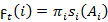
Probability distribution for symbol observation in state j is 


As it is representing the probability of observation symbol used in model at time t in state j.
The primary state distribution π= { }
}
 ]
] 
By combining above three elements, a hidden markov model is defined and represented as

Observation sequence is generated by using the appropriate values of the M, Y, F, S,  . The observation series is expressed as follows
Where x is the number of observation in the sequence and  is the each observation with one of the symbol W. There are different problems associated with HMMS as follow:
In evaluation problem, given the observation sequence and a model
 How well calculate P
  ), the possibility of the inspection series, specified the form. In assessment problem, sequence of observation and model is given; the task is to calculate the possibility that experimental series was created by model.
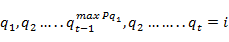
In learning with the observation sequence and the model  . How can we decide a equivalent status chain Q =
  2which is optimal in several significant sense. Hidden part of model is uncovered in this problem by finding the “correct” state sequence. Degenerate models, could not found “correct” sequence. Practically, an optimality principle is used to solve this difficulty.
In estimation problem adjusting the model parameters to maximize P ( ) Solving the problem the examination series use to alter the model parameter is called “training sequence”. Using trained observation it is possible to obtain optimal model parameters that create the best model.
Forward-Backward Algorithm
Forward Probabilities
For forward probalities following computations are required
Initialization:
 1
1
Induction:
 =
= 1
1
1
Termination:
P (A/ω) = 
Backward Probabilities
For computing the backward probabilities, we have to follow these steps
Initialization:
 = 1 1
= 1 1
Induction:
 =
=  t=X-1, X-2,...,1

Initially  which is most likely. In this form variable is defined as follows
 = P (
= P ( )
)
Viterbi Algorithm
A known method based on vibrant programming methods is used for decision particular best circumstances chain known as Viterbi algorithm. For only most excellent situation progression Q= { for specified study
(25)
It is defined to be
 =[
=[
 /ω] (26)
As equation (26) is calculated for t observations along a single path at time t and ends in state . The whole process used for ruling top status series can be declared as follow.
Initialization:
 (i) =
(i) =  1
1
 (i) = 0
Recursion:
 (j) =
(j) =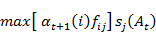 2
2
1
 (j) =
(j) =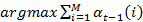 2
2
1
Termination:
 =
= (i)]
(i)]
 =
= (i)]
(i)]
Path (state sequence) backtracking:
 =
= t=X-1, X-2,…X
The difference between Viterbi and forward algorithm is just of summing and maximizing the calculations
Baum-Welch Algorithm
In HMM, for the estimation of model parameters a method is defined in which probability of observation sequence is maximizes. For this purpose select a model as ω= (F, S, π) So that P(A/ω) is maximized locally in Baum-Welch technique as it is alike to the EM (probability maximization) method. The iterative procedure is define λ(i,j), it is the chance of status  at moment t and state j at instant t+1, given the form and examination progression as
 = P (
= P (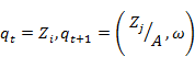
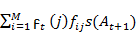
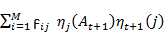
By using the definition of forward and backward variables, we be able to define λ(i,j) as follows.
λ(i, j) = 
= 
Now the model ω= (F, S, π) is helpful for the reestimation of parameters so the reestimated model is defined as 
3. LITERATURE REVIEW
Deng [1] proposed non stationary Hidden Markov models where every state was connected with different regression function of higher order with Gaussion process. They implemented and evaluated the special class of Hidden markov model. Model parameter of speech recognition included the standard stationary-state HMM. They developed a well-organized active programming technique which included optimization variable in combination with a state-dependent orthogonal polynomial regression method for estimating the model parameters. Such types of methods are applicable for speech information and finite-alphabets in speech process. Non-stationary state HMM superior to the usual stationary state HMM’s.
Crouse, et al. [2] introduced a technique for modeling the wavelet coefficients which are either independent or jointly Gaussian. Such type of models is impractical in many situations. Wavelet-domain hidden Markov models (HMMs) are useful for signal processing. Wavelet-domain HMMs are considered with the essential characteristics of the wavelet alter in mind and offer powerful, probability based signal models. For fitting the HMMs to observational signal data expectation maximization algorithms were developed. It is widely applicant for signal estimation, detection, classification, prediction, and also for synthesis. They developed the new techniques used in denoising, classification, and detection of signals.
Bahl [3] discussed that estimation of parameter can be done by hidden markov word models in speech process. They argued that estimating the parameters by maximum likelihood did not give the required accuracy and described another estimation method known as corrective training and proposed the minimum recognition errors. For linear classifiers corrective training correspondent to a procedure say error correcting training so used for adjusting the parameter values. Corrective training and maximum mutual information estimation are strongly parallel to each other. The evidences suggested that this method give the results more accurate and give significantly less errors than maximum likelihood estimation in recognition process.
Boreczky and Wilcox [4] described hidden markov models (HMM) technique for video segmentation. Video is partitioned into two regions say shooting limits and camera movement in taking shots.
Dangelmayr [5] used the algorithms to predict the future events from time series by generating maps. Transition probalities are computed and modeled. They applied this procedure in two types of data as Stochastic and Deterministic. Chaotic data estimated the quality of predictions. Prediction of chaotic and noisy time series is done.
Schliep, et al. [6] presented that the cellular processes cause changes over time. Reason behind the regulations can be observed and measured those changes over time. The essential time series data suggested that through clustering performance can be improved those dependencies. Use Hidden Markov Models (HMMs) to account dependencies along the time axis in time series data and also concern with missing values. As this method maximizes the joint likelihood of clustering and models and supporting partially supervised learning process, adding groups of labeled data in collection of clusters at the start. They also proposed a heuristic approach for determination of the number of clusters. They evaluated the method for yeast cell cycle and fibroblasts serum response datasets, and compare them with encouraging results, to the autoregressive curves method.
Ben and Marc [7] presented that observation data for communicable nosocomial pathogens usually consist of short time series of low numbered counts of infected patients. Dispersion and autocorrelation may occur in time series data. Inferences that depend on such analyses cannot be considered as reliable when patient-to-patient communication is important. They proposed a method for analyzing the data based on a mechanistic model of the plague process. They developed a ‘structured’ hidden Markov model is generated by a simple communication model. They applied both structured and standard (unstructured) hidden Markov models to time series for three important pathogens. They found that both methods can offer marked improvements more than currently used approaches
Hassan and Nath [8] presented hidden Markov models (HMM) approach for forecasting stock price. They applied HMM to forecast the airlines stock. HMMs have been extensively used for pattern recognition and classification problems. However, it is not very simple to use HMM for predicting future events. So they used only one HMM that is trained on the past dataset of the chosen airlines. By interpolating the neighboring values of the datasets forecasts were ready. The results obtained using HMM is hopeful and HMM offers a new pattern for stock market forecasting.
4. PROPOSED WORK
In this dissertation we represented hidden markov model in a very compact form as follow

Observation sequence is generated by using the appropriate values of the M, Y, F, S, . The observation sequence is expressed as follows
Where x is the number of observation in the sequence and  is the each observation with one of the symbol W.
We have presented our hidden markov model consisting of two states and one hidden state as bellow
Hidden Markov Model
Sequence
A sequence of observation symbols that is wearing sun glasses (hidden state) is generated. Its order is depending on the number of observation symbols used in the model. It is basis of emission matrix which further facilitate for computation of algorithm.
States of Model
As the states of the model are cloudy and partly cloudy coded as 1 and 2 respectively and shown as in the model above. As the states of the model build up the order of transition matrix which is very helpful for further analysis.
The sequence and states are taken from a known model, through specified changeover likelihood matrix and production likelihood matrix and we generated
An arbitrary chain ‘seq’ of emission signs.
A chance state series of ‘states’.
The extent of sequence as well as state is same.
In above Figure it is representing the hidden markov model as  and
and  are the two states of the model and
  ,
, and
and  is the observation sequence with probability
  ,
, ,
, with state 1 and
  ,
, and
and  with state 2.
In above Figure it is representing the hidden markov model as with state 2.
Forward Algorithm
For this procedure probabilities calculated are as
Table-4.1. forward probabilities
| No. of obs | Forward probabilities |
| [1-10] | |
| State 1 | 1.0000 0.1753 0.6380 0.3664 0.5218 0.4316 0.4835 0.4534 0.4708 0.4608 |
| State 2 | 0 0.8247 0.3620 0.6336 0.4782 0.5684 0.5165 0.5466 0.5292 0.5392 |
| [11-20] | |
| State 1 | 0.4666 0.4632 0.4652 0.4640 0.4647 0.4643 0.4645 0.4644 0.4645 0.4644 |
| State 2 | 0.5334 0.5368 0.5348 0.5360 0.5353 0.5357 0.5355 0.5356 0.5355 0.5356 |
| [21-30] | |
| State 1 | 0.4645 0.4644 0.4644 0.4644 0.4644 0.4644 0.4644 0.4644 0.4644 0.4644 |
| State 2 | 0.5355 0.5356 0.5356 0.5356 0.5356 0.5356 0.5356 0.5356 0.5356 0.5356 |
Source: software results
BACKWARD ALGORITHM
Backward probabilities are as follows
Table-4.2. backward probabilities
| No. of obs. | Backward probabilities |
| [1-10] | |
| State 1 | 1.0000 1.0699 1.0295 1.0528 1.0393 1.0471 1.0426 1.0452 1.0437 1.0446 |
| State 2 | 0.9208 0.9852 0.9480 0.9695 0.9571 0.9642 0.9601 0.9625 0.9611 0.9619 |
| [11-20] | |
| State 1 | 1.0441 1.0444 1.0442 1.0443 1.0443 1.0443 1.0443 1.0443 1.0443 1.0443 |
| State 2 | 0.9614 0.9617 0.9615 0.9616 0.9616 0.9616 0.9616 0.9616 0.9616 0.9616 |
| [21-30] | |
| State 1 | 1.0443 1.0443 1.0443 1.0443 1.0443 1.0443 1.0443 1.0443 1.0443 1.0443 |
| State 2 | 0.9616 0.9616 0.9616 0.9616 0.9616 0.9616 0.9616 0.9616 0.9616 0.9616 |
The State Sequence
The transition and emission matrices along with initial state probability vector are used in Viterbi algorithm to compute the most likely sequence of states the model.
Table-4.3. Likely states of the model
| [1-17] | 2 1 2 1 2 1 2 1 2 1 2 1 2 1 2 1 2 |
| [18-34] | 1 2 1 2 1 2 1 2 1 2 1 2 1 2 1 2 1 |
| [35-51] | 2 1 2 1 2 1 2 1 2 1 2 1 2 1 2 1 2 |
Estimation of Parameters
Parameters of the model estimated using the Baum Welch Algorithm is given as follows:
Table-4.4. estimated transition matrix
| States | cloudy | Partly cloudy |
| Cloudy | 0.244898 | 0.755102 |
| Partly cloudy | 0.74 | 0.26 |
In transition probability matrix, there is .244 probability of moving from cloudy state to cloudy state in next iteration. Algorithm gives probability of .74 moving from partly cloudy state to cloudy state. Transition matrix is satisfying the property that row sum should be equal to 1.
Table-4.5. estimated emission matrix
| Observation symbol | emission probability |
| Wear sunglasses | 0.5 |
| Not wear sunglasses | 0.5 |
There is 50% chance of wearing sunglasses in both the states as cloudy and partly cloudy.
So the new model is created by using these results
Where
 =
=
 =
=

M= two number of states in the model called cloudy and partly cloudy
Y=Number of Hidden state in the model called sunglasses
State Space Model
The inner state variables are the smallest probable division of system variables that can represent the whole state of the system at any specified instance. The minimum number of state variables required to represent a given system,  , is usually equal to the order of the system. The most general state-space representation of a linear system with p inputs, q outputs and M state variables is written in the following form.
Where
Y(t) is the state vector, Y(t) ϵ R.
X(t) is the output vector, X(t) ϵ R.
 is input or control vector.
F(y) is the state matrix.
S(x) is output matrix
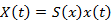
Prediction
After estimating the parameters we perform the prediction of states given in the model. For this purpose we predict 200 values and results are as follows
Figure-4.1. prediction
In the above figure prediction is done as each peak value is showing the each state. Graph is showing the transitions from one state to the second state.
In our study we run the algorithms to solve the problems related to the hidden markov model as the evaluation problem, learning problem, and estimating problem. As the evaluation problem is solved by using forward backward algorithm so as calculating the forward probabilities and backward probabilities. In this algorithm sequence is partitioned and forward backward probabilities are calculated as sum of both probabilities is same. Further more in learning problem tells us the likely state sequence followed by model as Viterbi algorithm is used for this purpose. Nextly estimation of parameters of model is done by Baum-Welch algorithm. We estimate the transition matrix and emission matrix through this procedure.
| Funding: This study received no specific financial support. |
| Competing Interests: The authors declare that they have no competing interests. |
| Contributors/Acknowledgement: All authors contributed equally to the conception and design of the study. |
REFERENCES
[1] L. Deng, "Speech recognition using hidden markov models with polynomial regression function as non-stationary states," IEEE Transactions on Speech and Audio Processing, vol. 2, pp. 507-520, 1994. View at Google Scholar | View at Publisher
[2] M. S. Crouse, R. D. Nowak, and R. G. Baraniuk, "Wavelet based statistical signal processing using hidden markov models," Signal Processing, IEEE, vol. 46, pp. 886-902, 1998. View at Google Scholar | View at Publisher
[3] L. Bahl, "A new algorithm for the estimation of hidden markov model parameters: Acoustics," Speech and signal Processing IEEE, vol. 1, pp. 493-497, 1988.
[4] J. S. Boreczky and L. D. Wilcox, "A hidden markov model framework for video segmentation using audio and image features, acoustics, speech and signal processing," Proceeding of IEEE, vol. 6, pp. 3741-3744, 1998.
[5] G. Dangelmayr, "Time series prediction by estimating markov probabilities through topology preserving maps," Proc SPIE, vol. 3812, pp. 86-93, 1999.
[6] A. Schliep, A. Schönhuth, and C. Steinhoff, "Using hidden markov model to analyze gene expression time course data," Bioinformatics, vol. 19, pp. i255-i263, 2003. View at Google Scholar | View at Publisher
[7] C. Ben and L. Marc, "The analysis of hospital infection data using hidden markov models," Biostatistics, vol. 5, pp. 223-237, 2004. View at Google Scholar | View at Publisher
[8] M. R. Hassan and B. Nath, "Stock market forecasting using hidden Markov model: A new approach," IIntelligent Systems Design and Applications, 2005. ISDA'05. Proceedings. 5th International Conference on. IEEE, 2005, pp. 192-196.
BIBLIOGRAPHY
[1] F. Alastair, "Prediction of wolf (Canis Lupus) kill-sites using hidden markov models," Ecological Modeling, vol. 97, pp. 237-246, 2006. View at Google Scholar | View at Publisher
| Views and opinions expressed in this article are the views and opinions of the author(s), Journal of Asian Scientific Research shall not be responsible or answerable for any loss, damage or liability etc. caused in relation to/arising out of the use of the content. |