


A STUDY ON HOST MORTALITY RATE OF A THREE SPECIES MULTI ECOLOGY WITH UNLIMITED RESOURCES FOR THE FIRST SPECIES

1Department of Mathematics, Chaitanya Group of Colleges,Hanamkonda, Telangana State, India
ABSTRACT
The purpose of this paper is to examine the stability analysis of a three species ecology with mortality rate for the host. The system comprises of a commensal (S1), two hosts S2 and S3 ie, S2 and S3 both benefit S1, without getting themselves affected either positively or adversely. Further the first species has unlimited resources. The model equations constitute a set of three first order non-linear coupled ordinary differential equations. Criteria for the asymptotic stability of all the four equilibrium states are established. Trajectories of the perturbations over the equilibrium states are illustrated and the global stability of the system is established with the aid of suitably constructed Liapunov’s function and finally fourth order Runge-Kutta method is applied to obtain numerical solutions of the growth rate equations.
© 2017 AESS Publications. All Rights Reserved.
Keywords: Commensal, Equilibrium state, Host, Trajectories, Neutrally stable, Stable, Unstable.
Article History: Received: 28 April 2017, Revised: 25 May 2017, Accepted: 29 May 2017, Published: 2 June 2017
Contribution/ Originality: The paper contributes the first logical analysis in biological investigations with an iterative procedure of information collection. If such models are properly developed and used, they can provide insight into the relations between the physical variables and process influencing the system being studied. The resulting interplay between the experimental investigation and the theoretical model can be an essential factor in designing experiments and in the interpretation of data.
1. INTRODUCTION
Ecology is a branch of life sciences connected to the existence of diverse species in the same environment and habitat. It is natural that two or more species living in a common habitat interact in different ways. Significant research in the area of theoretical ecology has been thresholded by Lotka [1] and by Volterra [2]. Several mathematicians and ecologists contributed to the growth of this area of knowledge. Mathematical ecology can be broadly divided into two main sub-divisions, Aut-ecology and Multi-ecology, which are described by several authors. Multi-ecology is an ecosystem comprised of two or more distinct species. Species interact with each other in one way or other. The Ecological interactions can be classified as Ammensalism, Competition, Commensalism, Neutralism, Mutualism, Predation, Parasitism and so on.
Mathematical modeling has been playing an important role for the last half a century in explaining several phenomena concerned with individuals and groups of populations in nature. The general concept of modeling has been presented in the monographs of Meyer [3]; Kushing [4]; Paul [5]; Kapur [6]. Srinivas [7] studied competitive ecosystem of two species and three species with limited and unlimited resources. Lakshmi [8]; Lakshmi and Pattabhiramacharyulu [9] studied prey-predator ecological models with partial cover for the prey and alternate food for the predator. Stability analysis of competitive species was carried out by Archana, et al. [10] and by Bhaskara and Pattabhiramacharyulu [11] while Ravindra [12] investigated mutualism between two species. Further Phani [13] studied some mathematical models of ecological commensalism. The present author [14-20] discussed on the stability of a three and four species multi-ecosystems.
The present investigation is on an analytical study of a three species (S1, S2, S3) multi ecology with mortality rate for the host and the first species has unlimited resources. The system comprises of a commensal (S1), two hosts S2 and S3 ie, S2 and S3 both benefit S1, without getting themselves affected either positively or adversely. Further S2 is a commensal of S3 and S3 is a host of both S1, S2. Commensalism is a symbiotic interaction between two populations where one population (S1) gets benefit from (S2) while the other (S2) is neither harmed nor benefited due to the interaction with (S1). The benefited species (S1) is called the commensal and the other (S2) is called the host. Some real-life examples of commensalism are presented below.
i. A squirrel in an oak tree gets a place to live and food for its survival, while the tree remains neither benefited nor harmed.
ii. A flatworm attached to the horse crab and eating the crab’s food, while the crab is not put to any disadvantage.
iii. Sucker fish (echeneis) gets attached to the under surface of sharks by its sucker. This provides easy transport for new feeding grounds and also food pieces falling from the sharks prey, to Echeneis.
2. METHODOLOGY
2.1. Notation
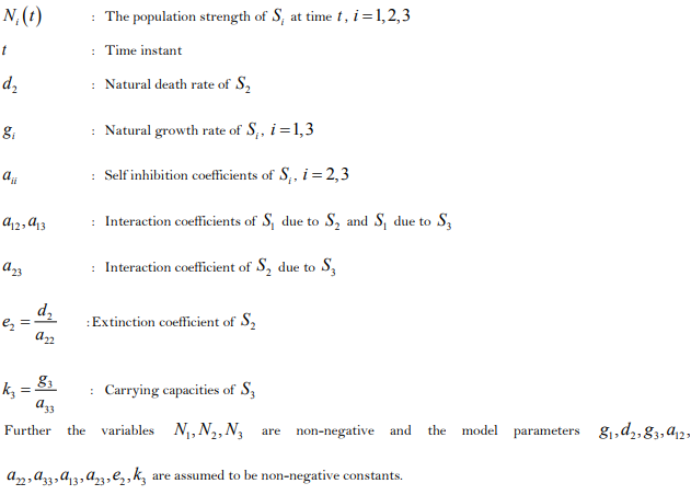
2.2. Theoretical Framework and Basic Equations
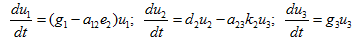
The model equations for the three species multi-ecosystem is given by the following system of first order non-linear ordinary differential equations.
(i) Equation for the first species ( ):
):
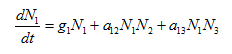 (1)
(1)
(ii) Equation for the second species ( ):
):
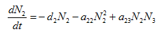 (2)
(2)
(iii) Equation for the third species ( ):
):
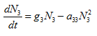 (3)
(3)
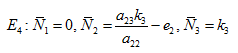
The system under investigation has four equilibrium states given by 
(i) Fully washed out state.
(ii) Only the third species is washed out and the other two are not.
(iii) Only the second species is washed out and the other two are not.
(iv) Only the first species is washed out and the other two are not.
2.3. Stability of the Equilibrium States
Let us consider small deviations from the steady state
i.e., 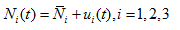 (4)
(4)
where  is a small perturbations in the species Si.
The basic equations are quasi-linearized over the equilibrium state  to obtain the equations for the perturbed state as
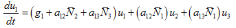 (5)
(5)
 (6)
(6)
 (7)
(7)
The characteristic equation for the system is
|A – λI| = 0 (8)
The equilibrium state is stable, if all the roots of the equation (8) are negative in case they are real or have negative real parts, in case they are complex.
2.3.1. The Stability of
The basic equations are quasi-linearized to obtain the equations as
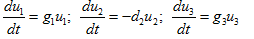 (9)
(9)
The characteristic equation is  (10)
(10)
The characteristic roots of (10) are  . Since two of these three roots are positive. Hence the state is unstable and the solutions of the equations (9) are
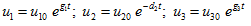 (11)
(11)
where  are the initial values of
  respectively.
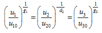
Trajectories of Perturbations
The trajectories in  and
and  planes are
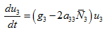
2.3.2. The Stability of
In this state, the basic equations can be quasi-linearized, we get
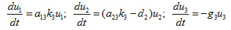 (12)
(12)
The characteristic roots are  . Since one of these three roots is positive, hence the state is unstable.
Case (i): When 
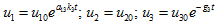
In this case, the solutions of (12) are
 (13)
(13)
Case (ii): When 
In this case, the solutions are given by
 (14)
(14)
Case (iii): When 
In this case, the solutions are
 (15)
(15)
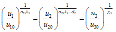
Trajectories of perturbations
The trajectories in the and planes are given by
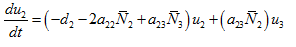
2.3.3. The Stability of
The basic equations can be quasi-linearized, we get
 (16)
(16)
The characteristic roots are 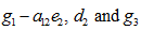 . Since two of these three roots are positive, hence the state is unstable.
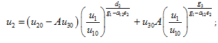
Case (i): When 
In this case, the equations (16) yield the solutions,
 (17)
(17)
where 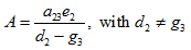 (18)
(18)
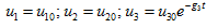
Case (ii): When 
In this case, the solutions of (16) are
 (19)
(19)
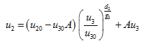
Case (iii): When 
In this case, the solutions are
 (20)
(20)
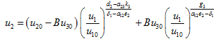
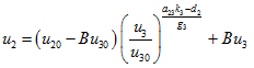
Trajectories of Perturbations
The trajectories in the and planes are
 ;
; 
2.3.4. The Stability of
In this state, the basic equations can be quasi-linearized,
We have
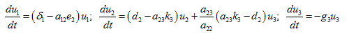 (21)
(21)
where 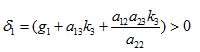 (22)
(22)
The characteristic roots are  . The equations (21) yield the solutions.
 (23)
(23)
where  (24)
(24)
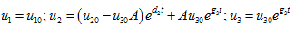
Case (i): When
In case all the three roots are negative, hence the state is stable. The solution (23) become
 (25)
(25)
Case (ii): When 
In case the state is neutrally stable and the solution (23) become
 (26)
(26)
Case (iii): When 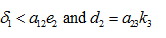
In case the state is neutrally stable and the solutions are 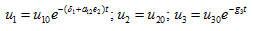 (27)
(27)
Case (iv): When 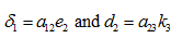
In case the state is neutrally stable and the solutions are given by
 (28)
(28)
Case (v): When 
In case the state is unstable and the equations (21) yield the solutions.
 (29)
(29)
Case (vi): When
In case the state is unstable and solutions are
(30)
Case (vii): When  or
or 
When 
In case the state is unstable.
Trajectories of perturbations
The trajectories in the and planes are given by
 ;
; 
3. LAPUNOV’S FUNCTION FOR GLOBAL STABILITY
In section 5 we discussed the local stability of all four equilibrium states. From which only one state  is stable and rest of them are unstable. We now examine the global stability of dynamical system (1), (2) and (3) at this state by suitable Liapunov’s function.
Theorem: The equilibrium state 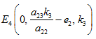 is globally asymptotically stable.
Proof: Let us consider the following Liapunov’s function
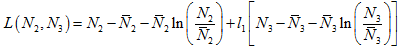 (31)
(31)
where l1 is a suitable constant to be determined as in the subsequent steps.
Now, the time derivative of L, along with solutions of (2) and (3) can be written as
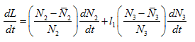 (32)
(32)
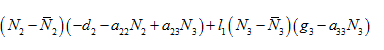
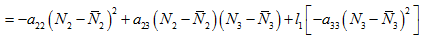
Choosing, 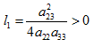 and with some algebraic manipulation, we get
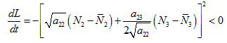 (33)
(33)
Hence, the steady state is globally asymptotically stable.
4. NUMERICAL EXAMPLES
The numerical solutions of the growth rate equations computed employing the fourth order Runge-Kutta method for specific values of the various parameters that characterize the model and the initial conditions. The results are illustrated in Figures from 1 to 6.
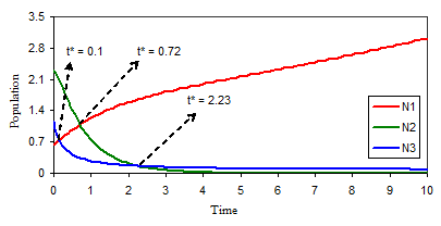
Figure-1. Variation of N1, N2, N3 against time (t) for g1 = 0.02, a12 = 0.28, a13 = 0.52, d2 = 1.46, a22 = 0.32, a23 = 1.64, g3 = 0.28, a33 = 3.52, N1 = 0.62, N2 = 2.32, N3 = 1.16.
Source: MS-Excel by using Runge-Kutta method
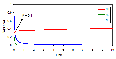
Figure-2. Variation of N1, N2, N3 against time (t) for g1 = 0.01, a12 = 5.16, a13 = 0.44, d2 = 8.64, a22 = 13.05, a23 = 0.45, g3 = 0.17, a33 = 23.53, N1 = 0.3, N2 = 0.2, N3 = 0.8.
Source: MS-Excel by using Runge-Kutta method
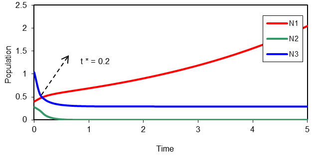
Figure-3. Variation of N1, N2, N3 against time (t) for g1 = 0.12, a12 = 3.96, a13 = 0.52, d2 = 17.76, a22 = 38, a23 = 33.24, g3 = 3.8, a33 = 13, N1 = 0.4, N2 = 0.28, N3 = 1.04.
Source: MS-Excel by using Runge-Kutta method
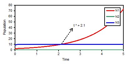
Figure-4. Variation of N1, N2, N3 against time (t) for g1 = 0.68, a12 = 1.72, a13 = 0.001, d2 = 24.52, a22 = 0.001, a23 = 0.4, g3 = 32.44, a33 = 3.32, N1 = 2.24, N2 = 0.4, N3 = 8.76.
Source: MS-Excel by using Runge-Kutta method
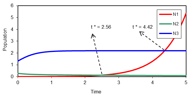
Figure-5. Variation of N1, N2, N3 against time (t) for g1 = 0.67, a12 = 7.8, a13 = 0.001, d2 = 2.3, a22 = 1.04, a23 = 1.04, g3 = 3.16, a33 = 1.44, N1 = 0.001, N2 = 0.28, N3 = 1.32.
Source: MS-Excel by using Runge-Kutta method
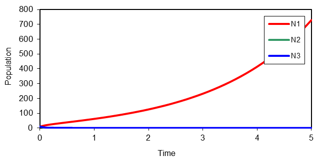
Figure-6. Variation of N1, N2, N3 against time (t) for g1 = 0.28, a12 = 0.8, a13 = 0.8, d2 = 10.72, a22 = 15.48, a23 = 1.84, g3 = 0.68, a33 = 2, N1 = 10, N2 = 10, N3 = 10.
Source: MS-Excel by using Runge-Kutta method
5. OBSERVATIONS OF THE ABOVE GRAPHS
6. CONCLUSION
The present paper deals with an investigation on the stability of a three species syn eco-system with mortality rate for the host. In this paper we established all possible equilibrium states. It is conclude that, in all four equilibrium states, only one state E4 is conditionally stable. Further the global stability is established with the help of suitable Liapunov’s function and the growth rates of the species are numerically estimated using Runge-Kutta fourth order method.
| Funding: This study received no specific financial support. |
| Competing Interests: The author declares that there are no conflicts of interests regarding the publication of this paper. |
REFERENCES
[1] A. J. Lotka, Elements of physical biology. Baltimore: Williams and Wilking, 1925.
[2] V. Volterra, Leconssen La Theorie Mathematique De La Leitte Pou Lavie. Paris: Gauthier-Villars, 1931.
[3] W. J. Meyer, Concepts of mathematical modeling: Mc.Grawhill, 1985.
[4] J. M. Kushing, Integro-differential equations and delay models in population dynamics. Lecture notes in bio-mathematics: Springer Verlag, 1977.
[5] C. A. Paul, Ecology. New York: John Wiley, 1986.
[6] J. N. Kapur, Mathematical modeling in biology & medicine: Affiliated East West, 1985.
[7] N. C. Srinivas, "Some mathematical aspects of modeling in bio-medical sciences," Ph.D. Thesis, Kakatiya University, 1991.
[8] N. K. Lakshmi, "A mathematical study of a prey-predator ecological model with a partial cover for the prey and alternate food for the predator," Ph.D. Thesis, JNTU, 2005.
[9] N. K. Lakshmi and N. C. Pattabhiramacharyulu, "A prey-predator model with cover for prey and alternate food for the predator and time delay," International Journal of Scientific Computing, vol. 1, pp. 7-14, 2007.
[10] R. R. Archana, N. C. Pattabhiramacharyulu, and G. B. Krisha, "A stability analysis of two competetive interacting species with harvesting of both the species at a constant rate," International Journal of Scientific Computing, vol. 1, pp. 57 - 68, 2007.
[11] R. S. B. Bhaskara and N. C. Pattabhiramacharyulu, "Stability analysis of two species competitive eco-system," International Journal of Logic Based Intelligent Systems, vol. 2, pp. 79 - 86, 2008.
[12] R. R. Ravindra, "A study on mathematical models of ecological mutualism between two interacting species," Ph.D. Thesis, O.U, 2008.
[13] K. N. Phani, "Some mathematical models of ecological commensalism," Ph.D. Thesis, ANU, 2010.
[14] P. B. Hari and N. C. Pattabhiramacharyulu, "On the stability of a four species: A prey-predator-host-commensal-syn eco-system-II," International e Journal of Mathematics and Engineering, vol. 5, pp. 60 - 74, 2010.
[15] P. B. Hari and N. C. Pattabhiramacharyulu, "On the stability of a four species: A prey-predator-host-commensal-syn eco-system-VII," International Journal of Applied Mathematical Analysis and Applications, vol. 6, pp. 85 - 94, 2011. View at Google Scholar
[16] P. B. Hari and N. C. Pattabhiramacharyulu, "On the stability of a four species: A prey-predator-host-commensal-syn eco-system-VIII," Advances in Applied Science, Research, vol. 2, pp. 197-206, 2011. View at Google Scholar
[17] P. B. Hari and N. C. Pattabhiramacharyulu, "On the stability of a four species syn eco-system with commensal prey predator pair with prey predator pair of hosts-V," International Journal of Open Problems in Computer Mathematics, vol. 4, pp. 129 - 145, 2011.
[18] P. B. Hari and C. N. Pattabhiramacharyulu, "On the stability of a four species syn eco-system with commensal prey predator pair with prey predator pair of hosts-VII (Host of S2 washed out states)," Journal of Communication and Computer, vol. 8, pp. 415 - 421, 2011. View at Google Scholar
[19] P. B. Hari and N. C. Pattabhiramacharyulu, "On the stability of a typical three species syn eco-system," International Journal of Mathematical Archive, vol. 3, pp. 3583-3601, 2012. View at Google Scholar
[20] P. B. Hari and N. C. Pattabhiramacharyulu, "On the stability of a four species syn eco-system with commensal prey predator pair with prey predator pair of hosts-VI," Matematika, vol. 28, pp. 181-192, 2012. View at Google Scholar
| Views and opinions expressed in this article are the views and opinions of the author(s), Journal of Asian Scientific Research shall not be responsible or answerable for any loss, damage or liability etc. caused in relation to/arising out of the use of the content. |